Welcome

How to cite this book

If you use this book in your work, please cite it as:

APA: Chaudhri, A. (2026). Seven Vector Databases in Seven Days. Self-published. https://seven-vector-databases.github.io/

BibTeX:

@online{chaudhri2026vectordatabases,
  author  = {Chaudhri, Akmal},
  title   = {Seven Vector Databases in Seven Days},
  year    = {2026},
  url     = {https://seven-vector-databases.github.io/},
  urldate = {2026-07-21}
}

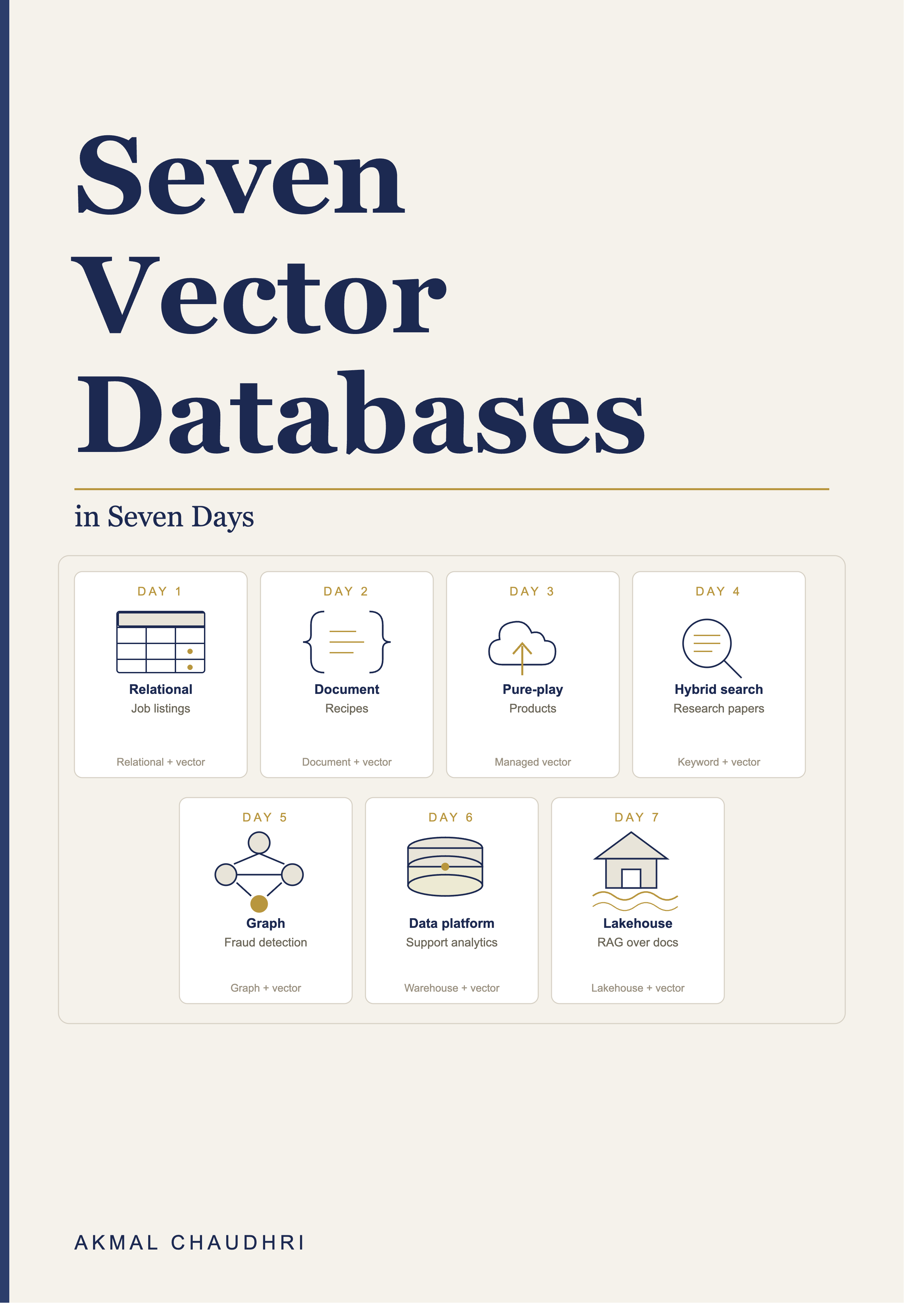
Cover

License

Copyright

Copyright © 2026 Akmal Chaudhri. All rights reserved.

Publication Information

First published: July 2026

The latest version of this book, together with updates, errata and additional resources, is available at:

seven-vector-databases.github.io

Book License

Seven Vector Databases in Seven Days is licensed under the Creative Commons Attribution-NonCommercial-NoDerivatives 4.0 International License (CC BY-NC-ND 4.0).

You are free to copy and redistribute this book in any medium or format under the following conditions:

• Attribution - You must give appropriate credit, provide a link to the license and indicate if changes were made.
• NonCommercial - You may not use the material for commercial purposes.
• NoDerivatives - If you remix, transform or build upon the material, you may not distribute the modified material.

The full license text is available at:

creativecommons.org/licenses/by-nc-nd/4.0

Code License

Unless otherwise stated, all code samples, notebooks, scripts and source files accompanying this book are licensed under the Apache License 2.0.

You are free to use, modify and redistribute this code, including for commercial purposes, subject to the terms of the Apache License 2.0.

The full license text is available at:

apache.org/licenses/LICENSE-2.0

This distinction means that the book’s written content is protected under the Creative Commons license, while the accompanying code remains freely available for use, modification and integration into your own projects.

Trademarks

Product names, company names and logos mentioned in this book may be trademarks or registered trademarks of their respective owners.

Their inclusion is for identification and educational purposes only and does not imply any affiliation with, sponsorship by or endorsement from the respective trademark holders. All trademarks remain the property of their respective owners.

Disclaimer

The information in this book, including all code samples, scripts and notebooks, is provided “as is” without warranty of any kind, express or implied.

The author makes no representations or warranties regarding the accuracy, completeness, reliability or suitability of the information contained herein for any particular purpose.

Examples are provided solely to illustrate technical concepts, database patterns and software architectures.

Readers are responsible for independently validating all code, configurations and recommendations before using them in production environments.

To the fullest extent permitted by law, the author shall not be liable for any direct, indirect, incidental, special, consequential or other damages arising from the use of or inability to use, the information, code or techniques described in this book.

About the Author

Akmal Chaudhri is a technical leader, educator and author with extensive experience in databases, AI and developer relations. He specializes in technical writing, developer education and community building, helping engineers and organizations understand and adopt complex technologies through clear, practical and engaging content. He is a frequent international speaker, a published author and a contributor to industry discussions on data platforms, AI and software development.

Today, Akmal works in developer education at Neo4j, where he focuses on technical content, workshops and community initiatives. While his professional role has evolved, this book represents an independent exploration of various data platforms.

Based in the United Kingdom, Akmal continues to work at the intersection of databases, AI and developer tooling, helping developers build modern data-driven applications.

For book updates, code samples and additional resources, visit the Book website.

To connect professionally or follow his latest work, visit LinkedIn.

Introduction

Why vector databases?

Something changed in software development around 2022. Applications began needing to search not just for exact matches - a user ID, a product SKU, a keyword - but for meaning. “Find me something like this.” “What documents are relevant to this question?” “Which past support tickets are similar to this one?” These aren’t keyword search problems. They’re similarity problems and the data structure that makes similarity search practical at scale is the vector embedding.

A vector embedding is a list of numbers - typically hundreds or thousands of them - that encodes the semantic meaning of a piece of text, an image or any other content. Two pieces of content with similar meanings will have embeddings that are close together in vector space, even if they share no words in common. This property is what makes it possible to ask “find me jobs related to building machine learning models in production” and get back relevant results even when the job listings use entirely different vocabulary.

Vector databases are systems built to store these embeddings and search across them efficiently. Some are purpose-built for the task. Others are general-purpose databases that have added vector search as a capability. The field has expanded rapidly and evaluating the options is now a real problem for teams building AI-powered features.

What this book is about

This book isn’t a comparison of vector databases. It won’t tell you which one is “best.” It won’t produce a ranking or a scorecard.

What it’ll do is show you what each of seven databases is genuinely good at and when you’d reach for it over the others. Each chapter focuses on a different database and a different use case, chosen specifically because the use case plays to that database’s strengths. The goal isn’t to pit them against each other but to give you the context to make a good decision when you’re evaluating tooling for your own problem.

The seven databases covered are:

The progression is deliberate. We start with the familiar - Postgres, which most developers already have - and move through a document database, two dedicated vector databases, a graph database and, finally, the major data platforms. By the end, you’ll have a clear picture of where vector search fits in each architecture and what trade-offs each approach involves.

Who this book is for

This book is written for developers, data engineers and architects who are evaluating vector database options for a real project. It assumes you’re comfortable with Python and SQL. It doesn’t assume any prior experience with vector databases, embeddings or machine learning.

If you’re building a RAG application and wondering whether to use Pinecone, pgvector or something else - this book is for you. If you have data in Snowflake or Databricks and are wondering whether you need a separate vector database - this book is for you. If you’re new to vector search and want a practical grounding before making architectural decisions - this book is for you.

How the book is structured

Each chapter follows the same structure:

• What is it - an honest characterization of the database, not a marketing summary
• When would you reach for it - the evaluator’s question answered upfront
• The use case - the specific scenario for that chapter, chosen to showcase the database’s strengths
• The data - the dataset used and why it fits
• Building the application - hands-on walkthrough with code, including gotchas we encountered along the way
• What you’d hit in production - honest notes on limitations, operational considerations and costs
• When to look elsewhere - the cases where this database is probably not the right choice

Every chapter comes with a Jupyter notebook. The notebooks are self-contained and independently runnable. They use all-minilm via Ollama for local embedding generation, which means no embedding API keys or costs in any chapter. Where a managed cloud service is required - MongoDB Atlas, Pinecone, Weaviate Cloud, Neo4j AuraDB, Snowflake and Databricks - a free tier or trial account is sufficient for all the examples in the book.

A note on the “seven days” format

The “seven days” framing is a nod to the tradition of books like Seven Languages in Seven Weeks and Seven Databases in Seven Weeks. The format carries a specific promise: enough depth to form a genuine opinion, structured as a journey rather than a reference. You’re not expected to read this book in seven calendar days, but each chapter is written to stand alone, so you can read them in order or jump to the chapters most relevant to your situation.

A note on embeddings

Throughout the book we use the all-minilm model via Ollama to generate embeddings. This model produces 384-dimensional vectors and runs entirely locally on your machine. It isn’t the most powerful embedding model available - OpenAI’s text-embedding-3-large or Cohere’s embed models would produce higher-quality embeddings - but it’s free, fast and consistent across all seven chapters, which makes it ideal for a tutorial context.

In production, the choice of embedding model matters and deserves its own evaluation. The model, the chunking strategy and the indexing approach all interact. This book focuses on the database layer; the embedding layer is a separate concern that we deliberately keep constant so the database differences are the variable.

Code and notebooks

All notebooks and source code are available at:

seven-vector-databases.github.io

Each notebook is self-contained. You’ll need Python, a virtual environment, classic Jupyter and Ollama installed locally. Specific prerequisites for each chapter, including versions, are documented at the top of the relevant notebook.

Day 1: PostgreSQL + pgvector

What is it?

PostgreSQL needs little introduction. It’s the world’s most widely deployed open-source relational database, with a history stretching back to the late 1980s and an ecosystem that spans virtually every programming language, cloud platform and deployment model imaginable. Developers reach for Postgres because it’s reliable, standards-compliant and extraordinarily capable - it handles relational data, JSON documents, full-text search and geospatial queries, all without leaving the database.

The pgvector extension adds one more capability to that list: native vector similarity search. Released in 2021 and now available on every major managed Postgres platform, pgvector introduces a VECTOR data type and the indexing structures needed to search across it efficiently. With a single CREATE EXTENSION command, a Postgres database becomes a vector database.

What makes this interesting isn’t that pgvector is the fastest or most feature-rich vector search implementation - it’s not. What makes it interesting is that it requires no new infrastructure, no new operational skills and no new mental model. If your application already runs on Postgres, vector search is one extension away.

When would you reach for it?

The clearest signal is existing Postgres data. If your application already stores its data in Postgres - user profiles, product catalogs, support tickets, documents - adding pgvector means vector search lives alongside those data in the same database. You can filter by salary, location, date or any other column in the same query that computes semantic similarity. No synchronization between databases, no dual writes, no operational overhead of a second system.

The second signal is team familiarity. A team that knows SQL and knows Postgres can be productive with pgvector immediately. There’s no new query language to learn, no new SDK to integrate and no new infrastructure to operate.

The third signal is scale. pgvector handles millions of vectors comfortably, which covers the majority of real-world use cases. If you’re building a general-purpose search engine over billions of documents, you’ll eventually need something more specialized. But for most applications - internal tools, product search, recommendation features, RAG pipelines over a bounded corpus - pgvector is more than sufficient.

The use case

For this chapter we’ll build a semantic job listing search engine. Users describe what they’re looking for in natural language - “I want to work on machine learning models in production” or “looking for a data pipeline and ETL role” - and the system returns the most relevant listings from the database.

This use case is a natural fit for Postgres. Job listings are structured data: they have titles, locations, salary ranges and skills lists, all of which are natural relational columns. But the richest signal for relevance is the free-text description, which is where vector search earns its place. By embedding each description and indexing the resulting vectors, we can match a user’s query against the meaning of a listing rather than just its keywords.

The relational advantage becomes clear when we add filters. A user who wants a data engineering role in New York with a minimum salary of $130,000 shouldn’t have to choose between semantic relevance and structured constraints. With pgvector, both happen in a single SQL query.

The data

We generate a synthetic dataset of job listings programmatically rather than using a fixed hardcoded list. This keeps the notebook self-contained and lets us scale to any number of listings by changing a single configuration variable.

Each listing is assembled from pools of roles, companies, US cities, salary bands, skills and description templates. The templates are domain-aware - data roles get data-flavored descriptions, machine learning roles get ML-flavored ones - which gives enough variation for meaningful semantic search.

The key fields are:

• title - the job title, e.g. “Senior Data Engineer”
• company - the hiring company
• location - a US city or “Remote”
• salary_min and salary_max - salary band in US dollars
• skills - an array of relevant technologies
• description - a short prose description of the role; this is what we embed

The description field is the one that carries semantic meaning. Everything else is structured metadata that we use for filtering.

Building the application

Prerequisites

To follow along you’ll need:

• PostgreSQL 16 installed locally (use Homebrew on a Mac)
• pgvector installed from source (see the note below)
• Ollama running locally with the all-minilm model pulled
• Python 3.12 with a virtual environment

Note: The Homebrew formula for pgvector installs cleanly but leaves an empty package on Apple Silicon Macs - the extension files simply aren’t present after installation. The workaround is to install from source, as shown below.

brew uninstall pgvector
git clone https://github.com/pgvector/pgvector.git
cd pgvector
make
make install

This compiles pgvector against the local Postgres installation and places the extension files in the correct location.

Note: A Homebrew Postgres installation doesn’t create a postgres superuser. Instead, it creates a role matching the Mac username. When connecting from Python, use os.environ.get("USER") rather than hardcoding "postgres".

Configuration

We’ll keep all tunable parameters in a single cell at the top of the notebook. NUM_JOBS controls the size of the generated dataset - 500 is a reasonable default for exploring search quality. RANDOM_SEED ensures the same dataset is generated on every run.

LLM_EMBEDDING = "all-minilm"
NUM_JOBS      = 500
RANDOM_SEED   = 42

Determine embedding dimensions

We’ll determine the embedding dimensions dynamically from a test embedding:

def get_embedding(text: str) -> list:
    response = ollama.embeddings(model = LLM_EMBEDDING, prompt = text)
    return response["embedding"]

test_embedding = get_embedding("senior data engineer with Python and Spark")
EMBEDDING_DIMS = len(test_embedding)
print(f"Embedding dimensions: {EMBEDDING_DIMS}")

Connect to PostgreSQL and enable pgvector

conn = psycopg2.connect(
    dbname = "postgres",
    user   = os.environ.get("USER"),
    host   = "localhost",
    port   = 5432
)

conn.autocommit = True
cursor = conn.cursor()

cursor.execute("CREATE EXTENSION IF NOT EXISTS vector;")
print("pgvector extension enabled.")

Generate the dataset

Rather than a hardcoded list, we’ll assemble listings from component pools. Each description is built from a template appropriate to the role’s domain:

random.seed(RANDOM_SEED)

ROLES = [
    {"title": "Senior Data Engineer",     "domain": "data", "salary_band": (130000, 160000)},
    {"title": "Machine Learning Engineer","domain": "ml",   "salary_band": (150000, 190000)},
    # ... further roles
]

DESCRIPTION_TEMPLATES = {
    "data": [
        "Build and maintain {system} for a {company_type} specializing in {domain}. "
        "Work closely with {team} to ensure data quality and reliability.",
        # ... further templates
    ],
    # ... further domains
}

def generate_description(domain: str) -> str:
    template = random.choice(DESCRIPTION_TEMPLATES[domain])
    return template.format(
        system       = random.choice(SYSTEMS_BY_DOMAIN[domain]),
        company_type = random.choice(COMPANY_TYPES),
        platform     = random.choice(PLATFORMS),
        team         = random.choice(TEAMS),
        domain       = random.choice(DOMAINS),
    )

def generate_job_listings(n: int) -> list:
    listings = []
    for _ in range(n):
        role   = random.choice(ROLES)
        domain = role["domain"]
        sal_min, sal_max = role["salary_band"]
        offset = random.choice([-10000, -5000, 0, 5000, 10000])
        listings.append({
            "title":       role["title"],
            "company":     random.choice(COMPANIES),
            "location":    random.choice(LOCATIONS),
            "salary_min":  sal_min + offset,
            "salary_max":  sal_max + offset,
            "skills":      random.choice(SKILLS_BY_DOMAIN[domain]),
            "description": generate_description(domain),
        })
    return listings

job_listings = generate_job_listings(NUM_JOBS)

Create the table

The table schema is straightforward. The embedding column uses the VECTOR({EMBEDDING_DIMS}) type, which matches the output dimensionality of all-minilm.

cursor.execute("DROP TABLE IF EXISTS job_listings;")

cursor.execute(f"""
    CREATE TABLE job_listings (
        id          SERIAL PRIMARY KEY,
        title       TEXT,
        company     TEXT,
        location    TEXT,
        salary_min  INTEGER,
        salary_max  INTEGER,
        skills      TEXT[],
        description TEXT,
        embedding   VECTOR({EMBEDDING_DIMS})
    );
""")

Generate embeddings and load data

We embed each job description using Ollama and insert the result alongside the structured fields. The tqdm progress bar gives useful feedback when loading larger datasets.

for job in tqdm(job_listings, desc = "Inserting listings"):
    embedding = get_embedding(job["description"])
    cursor.execute("""
        INSERT INTO job_listings
            (title, company, location, salary_min, salary_max, skills, description, embedding)
        VALUES (%s, %s, %s, %s, %s, %s, %s, %s)
    """, (
        job["title"], job["company"], job["location"],
        job["salary_min"], job["salary_max"], job["skills"],
        job["description"], str(embedding)
    ))

Create the vector index

pgvector supports two index types: IVFFlat and HNSW. We’ll use HNSW, which gives better recall and is the recommended default for most workloads. Note that we’ll create the index after loading data - building it incrementally during inserts is significantly slower for bulk loads.

cursor.execute("""
    CREATE INDEX ON job_listings
    USING hnsw (embedding vector_cosine_ops);
""")

Semantic search

We embed the user’s query and find the most similar job descriptions using the <=> cosine distance operator.

def search_jobs(query: str, top_k: int = 5):
    query_embedding = get_embedding(query)
    cursor.execute("""
        SELECT title, company, location, salary_min, salary_max,
               1 - (embedding <=> %s::vector) AS similarity
        FROM job_listings
        ORDER BY embedding <=> %s::vector
        LIMIT %s;
    """, (str(query_embedding), str(query_embedding), top_k))

    results = cursor.fetchall()
    print(f"\nQuery: '{query}'\n")
    for title, company, location, sal_min, sal_max, similarity in results:
        print(f"  {title} @ {company} - {location}")
        print(f"  ${sal_min:,} - ${sal_max:,} | Similarity: {similarity:.3f}\n")

Running a few queries against the 500-listing dataset:

search_jobs("I want to work on machine learning models in production")

Query: 'I want to work on machine learning models in production'

  ML Ops Engineer @ RetailIQ - Phoenix, AZ
  $135,000 - $165,000 | Similarity: 0.717

  Machine Learning Engineer @ EdgeCore - Portland, OR
  $155,000 - $195,000 | Similarity: 0.700

  Prompt Engineer @ InsightCo - Portland, OR
  $110,000 - $140,000 | Similarity: 0.692

  Computer Vision Engineer @ GrowthLab - Austin, TX
  $140,000 - $175,000 | Similarity: 0.669

  ML Ops Engineer @ AlphaEdge - Austin, TX
  $140,000 - $170,000 | Similarity: 0.634

The relational advantage - filtered search

This is where Postgres genuinely earns its place. We combine semantic similarity with standard SQL filters in a single query. The key subtlety in the implementation is parameter ordering - the first embedding parameter appears in the SELECT clause, the filter parameters follow in the WHERE clause and the second embedding parameter appears in the ORDER BY.

def search_jobs_filtered(query: str, location: str = None, min_salary: int = None, top_k: int = 5):
    query_embedding = get_embedding(query)
    embedding_str   = str(query_embedding)

    filters       = []
    filter_params = []

    if location:
        filters.append("location ILIKE %s")
        filter_params.append(f"%{location}%")
    if min_salary:
        filters.append("salary_min >= %s")
        filter_params.append(min_salary)

    where_clause = "WHERE " + " AND ".join(filters) if filters else ""

    # First embedding param goes before the WHERE filters; second after (ORDER BY)
    params = [embedding_str] + filter_params + [embedding_str, top_k]

    cursor.execute(f"""
        SELECT title, company, location, salary_min, salary_max,
               1 - (embedding <=> %s::vector) AS similarity
        FROM job_listings
        {where_clause}
        ORDER BY embedding <=> %s::vector
        LIMIT %s;
    """, params)

A filtered search for technical leadership roles in New York with a minimum salary of $130,000:

search_jobs_filtered(
    "technical leadership and system design",
    location = "New York",
    min_salary = 130000
)

query = 'technical leadership and system design', location = 'New York', min_salary = $130,000

  Engineering Manager @ GrowthLab - New York, NY
  $175,000 - $215,000 | Similarity: 0.449

  Engineering Manager @ BridgeIT - New York, NY
  $175,000 - $215,000 | Similarity: 0.449

  Site Reliability Engineer @ DocuCraft - New York, NY
  $140,000 - $175,000 | Similarity: 0.336

  Search Engineer @ Orbis Cloud - New York, NY
  $135,000 - $165,000 | Similarity: 0.294

  NLP Engineer @ Orbis Cloud - New York, NY
  $135,000 - $170,000 | Similarity: 0.272

The SQL filter and the vector similarity operate together in a single round trip to the database. There’s no second system to query, no results to merge and no metadata to synchronize.

What you’d hit in production

Index build time. HNSW indexes are built at insert time, which slows bulk loads considerably. For large datasets, always load data first and create the index afterwards. The difference can be an order of magnitude.

Dimensionality limit. pgvector can index vectors of up to 2,000 dimensions, although the VECTOR type itself can store more. Most embedding models are well within the indexing limit - all-minilm produces 384 dimensions, OpenAI’s text-embedding-3-small produces 1,536. The exception is text-embedding-3-large at 3,072 dimensions, which requires dimensionality reduction before indexing.

Approximate vs exact search. HNSW is an approximate nearest neighbor algorithm. For the vast majority of applications this is fine - recall is high and the speed improvement over exact search is substantial. If you need guaranteed exact results, omit the index and use a sequential scan, but be aware this doesn’t scale beyond a few hundred thousand vectors.

Connection pooling. Vector queries are memory-intensive, particularly at higher dimensions. In production, use PgBouncer or a connection pooler to avoid connection exhaustion under load.

When to look elsewhere

pgvector is a strong default, but it isn’t the right choice for every situation. Consider a dedicated vector database if:

• You’re storing tens of millions of vectors and need sub-10ms retrieval at scale. Dedicated vector databases are built around this problem in a way that a general-purpose database with an extension is not.
• You need advanced filtering on high-cardinality metadata without index performance trade-offs. pgvector’s HNSW index applies the vector search first and filters afterwards, which can degrade precision when filters are highly selective.
• Your team has no existing Postgres footprint and no appetite for managing it. The operational simplicity argument only holds if Postgres is already in your stack.
• You need built-in embedding model integrations, multi-tenancy, namespacing or other features that dedicated vector databases provide out of the box.

For most applications - particularly those already running on Postgres - pgvector is the right place to start. It’s free, battle-tested and keeps your architecture simple. The chapters that follow explore what you gain by moving to a dedicated vector database and when that trade-off is worth making.

Day 2: MongoDB Atlas

What is it?

MongoDB is the world’s most popular document database. Rather than storing data in rows and columns, MongoDB stores it as documents - flexible, JSON-like structures that can hold nested objects, arrays and variably-shaped data without a fixed schema. This makes it a natural fit for content that doesn’t conform cleanly to a relational table, such as product catalogs with varying attributes, user profiles with optional fields or recipes with ingredient lists of different lengths.

MongoDB Atlas is the fully managed cloud version of MongoDB, available on AWS, GCP and Microsoft Azure. Atlas Vector Search extends Atlas with native vector similarity search, letting us store and query embeddings directly alongside our existing document data. There’s no separate vector store to maintain, no synchronization between systems and no new operational model to learn.

When would you reach for it?

The clearest signal is an existing MongoDB footprint. If an application already stores its data as documents in MongoDB, Atlas Vector Search is the path of least resistance - vector search becomes a field on existing documents rather than a reason to introduce a new database.

The second signal is variably structured content. Documents whose shape varies from record to record - recipes with different numbers of ingredients, products with different attribute sets, support tickets with optional fields - fit the document model naturally. In a relational database, this kind of variation requires either nullable columns, separate tables or JSON columns. In MongoDB it’s just how documents work.

The third signal is the aggregation pipeline. MongoDB’s query model is built around composable pipeline stages. The $vectorSearch stage plugs into this pipeline naturally, meaning we can chain vector search with filtering, grouping, lookup joins and projection in a single query. Developers already familiar with MongoDB’s aggregation model will find Atlas Vector Search intuitive to work with.

The use case

For this chapter we’ll build a semantic recipe finder. Users describe what they feel like eating in natural language - “something warm and spicy for a cold evening” or “a light fresh dish with vegetables for summer” - and get relevant recipes in return.

Recipes are a natural fit for the document model. Each recipe has a name, a cuisine, a difficulty rating, a prep time and an ingredient list - but the ingredient list varies in length from recipe to recipe and the set of attributes that matter differs by dish type. In a relational database this variability requires workarounds. In MongoDB it’s simply a document with an array field.

The description field on each recipe is a short prose summary of the dish. This is what we’ll embed and search over. The structured fields - cuisine, difficulty, prep time - serve as filters.

The data

We’ll generate recipes programmatically from pools of cuisines, cooking methods, ingredients and description templates. Each description is assembled from randomly selected components, giving enough variation for meaningful semantic search across hundreds of recipes.

The key fields are:

• name - the recipe name, e.g. “Korean Chicken And Green Beans”
• cuisine - the cuisine type, e.g. “Korean”, “Italian”, “Thai”
• difficulty - “Easy”, “Medium” or “Hard”
• prep_time - preparation time in minutes
• ingredients - a list of ingredients of varying length
• description - a short prose summary of the dish; this is what’s embedded

Note that ingredients is a list field with no fixed length. This is the document model working as intended - no schema changes are needed to accommodate recipes with a handful of ingredients or a dozen.

Building the application

Prerequisites

To follow along you’ll need:

• A MongoDB Atlas account
• Ollama running locally with the all-minilm model pulled
• Python 3.12 with a virtual environment

Create a free MongoDB Atlas cluster

If you don’t already have a cluster:

1. Go to MongoDB Atlas and create a free account
2. Once logged in, select Create a free starter database
3. Give the cluster a name (e.g. recipes)
4. Click Set it up for me
5. Copy and save database user credentials
6. Select Choose a connection method > Drivers > Python
7. Note down the connection string that looks like mongodb+srv://<username>:<password>@recipes.xxxxx.mongodb.net
8. From the left navigation pane select SECURITY > Database & Network Access
9. From the left navigation pane select NETWORK ACCESS > IP Access List
10. Add 0.0.0.0/0 for temporary open access during development

Configuration

We’ll set the following environment variable before running the notebook:

export MONGODB_URI="mongodb+srv://<username>:<password>@recipes.xxxxx.mongodb.net"

Then in the notebook:

MONGODB_URI   = os.environ["MONGODB_URI"]
DB_NAME       = "recipes_db"
COLLECTION    = "recipes"
INDEX_NAME    = "vector_index"
LLM_EMBEDDING = "all-minilm"
NUM_RECIPES   = 200
RANDOM_SEED   = 42

Note: NUM_RECIPES controls the size of the generated dataset. 200 is the recommended default for this chapter - embedding generation runs locally via Ollama and is single-threaded, so larger values will work but will take proportionally longer. Production pipelines would typically use a hosted embedding endpoint with async or batched generation to handle scale.

Determine embedding dimensions

We’ll determine the embedding dimensions dynamically from a test embedding:

def get_embedding(text: str) -> list:
    response = ollama.embeddings(model = LLM_EMBEDDING, prompt = text)
    return response["embedding"]

test_embedding = get_embedding("a warm spicy dish with chicken")
EMBEDDING_DIMS = len(test_embedding)
print(f"Embedding dimensions: {EMBEDDING_DIMS}")

Generate the dataset

We’ll assemble recipes from component pools - cuisines, cooking methods, proteins, vegetables, bases and description templates. The description templates are parameterized so each recipe gets a unique prose summary:

DESCRIPTION_TEMPLATES = [
    "{method} {protein} served over {base} with {vegetable}, {flavor} and perfect for {occasion}.",
    "A {flavor} {cuisine} dish featuring {method} {protein} with {vegetable} on a bed of {base}.",
    "{cuisine} classic: {method} {protein} with {vegetable}, {flavor} flavors ideal for {occasion}.",
    # ... further templates
]

def generate_recipe() -> dict:
    cuisine  = random.choice(CUISINES)
    method   = random.choice(COOKING_METHODS)
    protein  = random.choice(PROTEINS)
    veg      = random.choice(VEGETABLES)
    base     = random.choice(BASES)

    name = random.choice(RECIPE_NAME_TEMPLATES).format(
        cuisine = cuisine, method = method.capitalize(),
        protein = protein, vegetable = veg, base = base
    )

    description = random.choice(DESCRIPTION_TEMPLATES).format(
        cuisine = cuisine, method = method, protein = protein,
        vegetable = veg, base = base,
        flavor = random.choice(FLAVORS),
        occasion = random.choice(OCCASIONS),
    )

    return {
        "name":        name.title(),
        "cuisine":     cuisine,
        "difficulty":  random.choice(DIFFICULTIES),
        "prep_time":   random.choice(PREP_TIMES),
        "ingredients": list(set([protein, veg, base] + random.sample(VEGETABLES + PROTEINS, random.randint(2, 9)))),
        "description": description,
    }

recipes = [generate_recipe() for _ in range(NUM_RECIPES)]

Generate embeddings and load data

We’ll embed each recipe description and store the vector as an embedding field on the document:

collection.drop_search_index(INDEX_NAME)
collection.delete_many({})

documents = []
for recipe in tqdm(recipes, desc = "Generating embeddings"):
    doc = recipe.copy()
    doc["embedding"] = get_embedding(recipe["description"])
    documents.append(doc)

collection.insert_many(documents)

Create the vector index

We create the index programmatically using SearchIndexModel. The EMBEDDING_DIMS variable ensures the index definition stays in sync with whichever embedding model is in use:

search_index_model = SearchIndexModel(
    definition = {
        "fields": [
            {
                "type": "vector",
                "path": "embedding",
                "numDimensions": EMBEDDING_DIMS,
                "similarity": "cosine"
            },
            {
                "type": "filter",
                "path": "cuisine"
            },
            {
                "type": "filter",
                "path": "difficulty"
            },
            {
                "type": "filter",
                "path": "prep_time"
            }
        ]
    },
    name = INDEX_NAME,
    type = "vectorSearch"
)

collection.create_search_index(model = search_index_model)
print(f"Index '{INDEX_NAME}' creation initiated.")

Wait for the vector index to be ready

Note: Atlas Vector Search can report the index status as READY slightly before queries return results. A fixed delay isn’t reliable - even our small collection took around 30 seconds to become ready, and a larger one may need longer. The most robust approach is to poll the index status and then confirm with a test query.

After inserting data, confirm that the vector index we created is active.

print("Waiting for vector index to be active...")
while True:
    indexes = list(collection.list_search_indexes())
    status  = next((idx["status"] for idx in indexes if idx["name"] == INDEX_NAME), None)
    if status == "READY":
        print(f"Index '{INDEX_NAME}' is active.")
        break
    print(f"  Status: {status} - waiting...")
    time.sleep(5)

# Confirm the index is genuinely ready by running a test query
print("Confirming index is ready...")
while True:
    test = list(collection.aggregate([
        {
            "$vectorSearch": {
                "index":         INDEX_NAME,
                "path":          "embedding",
                "queryVector":   get_embedding("test"),
                "numCandidates": 10,
                "limit":         1,
            }
        }
    ]))
    if test:
        print("Index is ready.")
        break
    print("  Index not yet propagated - waiting...")
    time.sleep(5)

The second loop issues a real vector query and waits until it returns a result. This is the most reliable signal that the index is ready for use.

Semantic search

Atlas Vector Search uses MongoDB’s aggregation pipeline. The $vectorSearch stage takes a query vector and returns the most similar documents, ranked by cosine similarity. The $project stage controls which fields are returned and adds the similarity score via $meta: "vectorSearchScore".

def search_recipes(query: str, top_k: int = 5):
    query_embedding = get_embedding(query)

    pipeline = [
        {
            "$vectorSearch": {
                "index":         INDEX_NAME,
                "path":          "embedding",
                "queryVector":   query_embedding,
                "numCandidates": top_k * 10,
                "limit":         top_k,
            }
        },
        {
            "$project": {
                "_id":         0,
                "name":        1,
                "cuisine":     1,
                "difficulty":  1,
                "prep_time":   1,
                "description": 1,
                "score": {"$meta": "vectorSearchScore"},
            }
        }
    ]

    results = list(collection.aggregate(pipeline))
    print(f"\nQuery: '{query}'\n")
    for r in results:
        print(f"  {r['name']} ({r['cuisine']})")
        print(f"  {r['difficulty']} - {r['prep_time']} mins | Score: {r['score']:.3f}")
        print(f"  {r['description']}")
        print()

The numCandidates parameter controls how many documents Atlas considers before returning the top limit results. A higher value improves recall at the cost of latency. We use a ratio of 10x here because the collection is small, but the Atlas documentation recommends starting at 20x.

The document advantage - filtered search

Atlas Vector Search supports pre-filtering directly in the $vectorSearch stage. Filters are applied before the vector search, meaning only matching documents are considered as candidates. This is more precise than post-filtering and produces better results when filters are selective.

The filter fields must be declared in the index definition. We included cuisine, difficulty and prep_time when we created the index, so all three are available as filters:

def search_recipes_filtered(
    query:      str,
    cuisine:    str = None,
    difficulty: str = None,
    max_time:   int = None,
    top_k:      int = 5
):
    query_embedding = get_embedding(query)

    filter_doc = {}
    if cuisine:
        filter_doc["cuisine"]    = {"$eq": cuisine}
    if difficulty:
        filter_doc["difficulty"] = {"$eq": difficulty}
    if max_time:
        filter_doc["prep_time"]  = {"$lte": max_time}

    vector_search_stage = {
        "$vectorSearch": {
            "index":         INDEX_NAME,
            "path":          "embedding",
            "queryVector":   query_embedding,
            "numCandidates": top_k * 10,
            "limit":         top_k,
        }
    }
    if filter_doc:
        vector_search_stage["$vectorSearch"]["filter"] = filter_doc

    pipeline = [vector_search_stage, {"$project": {...}}]
    results  = list(collection.aggregate(pipeline))

Here is an example filtered search - “easy Italian recipes ready in 30 minutes or less”:

search_recipes_filtered(
    "a comforting pasta dish",
    cuisine    = "Italian",
    difficulty = "Easy",
    max_time   = 30
)

query = 'a comforting pasta dish', cuisine = 'Italian', difficulty = 'Easy', max_time = 30 mins

  Steamed Lamb With Zucchini (Italian)
  Easy - 20 mins | Score: 0.749
  steamed lamb served over tortillas with zucchini, creamy and comforting and perfect for meal prep.

  Poached Chicken With Mushrooms (Italian)
  Easy - 20 mins | Score: 0.702
  Simple and satisfying - poached chicken tossed with mushrooms and flatbread, light and fresh.

  Chickpeas And Roasted Peppers Noodles Bowl (Italian)
  Easy - 15 mins | Score: 0.676
  Quick and zesty and vibrant: pan-fried chickpeas with roasted peppers over noodles, great for a dinner party.

The function asks for up to five results, but only three come back because only three of the 200 recipes match all three filters.

Querying the document model

One of MongoDB’s strengths is querying nested and array fields directly. We can find all recipes containing a specific ingredient using a standard MongoDB query - no joins and no separate table, as follows:

def find_by_ingredient(ingredient: str, limit: int = 5):
    results = collection.find(
        {"ingredients": {"$in": [ingredient]}},
        {"_id": 0, "name": 1, "cuisine": 1, "difficulty": 1, "prep_time": 1, "ingredients": 1}
    ).limit(limit)

This works because ingredients is a native array field on the document. On a collection this small a scan is fine, but at scale we’d create a multikey index on ingredients, which MongoDB builds when we index an array field.

What you’d hit in production

Index propagation delay. As noted above, Atlas can report the index status as READY slightly before queries return results, and even our small collection took around 30 seconds to become ready. Budget for this in any automated pipeline that creates a collection and immediately queries it.

numCandidates tuning. The ratio between numCandidates and limit affects both recall and latency. Atlas documentation recommends at least limit * 20 and no more than 10,000. We use 10x here because the collection is small, and high-precision use cases may need higher values.

Filter field declaration. Filter fields must be declared in the index definition at creation time. Adding a new filterable field requires rebuilding the index. Plan your filter fields upfront.

Free tier limits. Atlas Free clusters support vector search but are intended primarily for development and testing. A Free cluster limits how many search indexes you can create, so check the current limits for your cluster tier. Vector indexes can contain up to 8,192 dimensions. For production deployments, MongoDB recommends using a dedicated cluster (M10 or higher).

Index management. The vector search index can be created, updated and dropped entirely from Python using SearchIndexModel and create_search_index() - no Atlas UI required. This makes the full lifecycle scriptable and repeatable.

When to look elsewhere

MongoDB Atlas is a strong choice when your application already runs on MongoDB or when your data are naturally document-shaped. Consider a dedicated vector database if:

• You have no existing MongoDB footprint and no other reason to run it. The operational simplicity argument only holds if MongoDB is already in your stack.
• You need the highest possible vector search performance at very large scale. Dedicated vector databases are built exclusively around this problem and can outperform a general-purpose database with vector search added on.
• Your data are highly relational with many joins. MongoDB handles references between documents, but deeply relational data are more naturally expressed in a relational database.
• You need advanced vector index configuration beyond what Atlas exposes. Dedicated vector databases offer more granular control over index parameters, distance metrics and quantization.

For teams already building on MongoDB, Atlas Vector Search is the natural path - it keeps the stack simple and lets vector search grow with the application without introducing a second system to operate.

Day 3: Pinecone

What is it?

Pinecone is a fully managed, purpose-built vector database. Unlike Day 1 and Day 2, where vector search was an extension or add-on to an existing database, Pinecone exists solely to store and search vectors. There’s no relational layer, no document model and no infrastructure to manage - just an API.

This is a deliberate design choice. Pinecone’s thesis is that vector search is a distinct enough problem to warrant its own dedicated system and that the operational overhead of running and tuning a general-purpose database is unnecessary friction when all you need is similarity search. You provision an index, upsert vectors, query them and let Pinecone handle everything else.

Pinecone organizes vectors in indexes. Each index stores vectors of a fixed dimension alongside optional metadata - structured fields like category, price or brand that can be used for filtering at query time. There are no tables and no schemas. The data model is intentionally minimal: an id, a vector and a metadata dictionary.

When would you reach for it?

The clearest signal is a pure vector search use case with no need for a broader data model. If your application needs to find similar items - products, documents, images, user profiles - and the structured filtering you need can be expressed as metadata on the vector record, Pinecone is a strong fit.

The second signal is managed simplicity. Pinecone requires no infrastructure decisions, no index tuning and no operational runbook. You don’t choose instance sizes, manage disk or worry about replication. For teams that want vector search without a dedicated infrastructure engineer, this is the value proposition.

The third signal is scale. Pinecone is built to handle hundreds of millions of vectors with consistent low-latency retrieval. If your use case will grow beyond what a general-purpose database with a vector extension can handle, Pinecone is designed for that ceiling.

The use case

For this chapter we’ll build a semantic product search engine for an electronics store. Users describe what they’re looking for in natural language - “a laptop for video editing under $1500” or “noise canceling headphones for travel” - and get relevant products in return.

This is a natural fit for Pinecone. Product search is a pure similarity problem: given a query, find the most semantically relevant items. The structured constraints a user might apply - category, price ceiling, performance tier - map naturally to Pinecone’s metadata filtering. There’s no relational data to join, no document hierarchy to navigate and no schema to maintain.

The data

We generate electronics product listings programmatically from pools of categories, brands, performance tiers, use cases and description templates. Each product has a name, category, brand, price, performance tier and a short prose description. The description is what we embed and search over. Everything else is stored as metadata on the vector record for filtering.

The key fields are:

• name - the product name, e.g. “VisionCore Laptop 576”
• category - e.g. “Laptop”, “Headphones”, “Camera”
• brand - one of fifteen fictional brands
• price - a realistic price for the category in US dollars
• performance - “entry-level”, “mid-range”, “high-performance”, “professional-grade” or “flagship”
• use_case - the intended audience, e.g. “remote workers”, “content creators”, “travelers”
• description - a short prose summary assembled from templates; this is what we embed

Building the application

Prerequisites

To follow along you’ll need:

• A Pinecone account with an API key
• Ollama running locally with the all-minilm model pulled
• Python 3.12 with a virtual environment

Configuration

We’ll set the following environment variable before running the notebook:

export PINECONE_API_KEY="your-api-key"

Then in the notebook:

PINECONE_API_KEY = os.environ["PINECONE_API_KEY"]
INDEX_NAME       = "electronics"
CLOUD            = "aws"
REGION           = "us-east-1"
LLM_EMBEDDING    = "all-minilm"
NUM_PRODUCTS     = 200
RANDOM_SEED      = 42

Note: NUM_PRODUCTS controls the size of the generated dataset. 200 is the recommended default for this chapter - embedding generation runs locally via Ollama and is single-threaded, so larger values will work but will take proportionally longer. Production pipelines would typically use a hosted embedding endpoint with async or batched generation to handle scale.

Determine embedding dimensions

We’ll determine the embedding dimensions dynamically from a test embedding:

def get_embedding(text: str) -> list:
    response = ollama.embeddings(model = LLM_EMBEDDING, prompt = text)
    return response["embedding"]

test_embedding = get_embedding("noise canceling headphones for travel")
EMBEDDING_DIMS = len(test_embedding)
print(f"Embedding dimensions: {EMBEDDING_DIMS}")

Connect to Pinecone

pc = Pinecone(api_key = PINECONE_API_KEY)
print("Connected to Pinecone.")

Generate the dataset

We assemble products from component pools. Description templates are parameterized to produce varied prose across all 200 products:

DESCRIPTION_TEMPLATES = [
    "A {performance} {category} designed for {use_case}, featuring {feature1} and {feature2}.",
    "Built for {use_case}, this {performance} {category} delivers {feature1} alongside {feature2}.",
    "The {brand} {category} is a {performance} option for {use_case}, offering {feature1} and {feature2}.",
    # ... further templates
]

def generate_product() -> dict:
    category    = random.choice(CATEGORIES)
    brand       = random.choice(BRANDS)
    performance = random.choice(PERFORMANCE)
    use_case    = random.choice(USE_CASES)
    features    = random.sample(FEATURES[category], 2)
    price_min, price_max = PRICE_BANDS[category]
    price       = round(random.randint(price_min, price_max) / 10) * 10

    description = random.choice(DESCRIPTION_TEMPLATES).format(
        category    = category,
        brand       = brand,
        performance = performance,
        use_case    = use_case,
        feature1    = features[0],
        feature2    = features[1],
    )

    return {
        "name":        f"{brand} {category} {random.randint(100, 999)}",
        "category":    category,
        "brand":       brand,
        "price":       price,
        "performance": performance,
        "use_case":    use_case,
        "description": description,
    }

products = [generate_product() for _ in range(NUM_PRODUCTS)]

Create the Pinecone index

We create a serverless index programmatically. If the index already exists from a previous run, we delete it and recreate it for a clean start. The EMBEDDING_DIMS variable ensures the index dimension matches the embedding model.

existing_indexes = [idx.name for idx in pc.list_indexes()]

if INDEX_NAME in existing_indexes:
    print(f"Deleting existing index '{INDEX_NAME}'...")
    pc.delete_index(INDEX_NAME)

print(f"Creating index '{INDEX_NAME}'...")
pc.create_index(
    name      = INDEX_NAME,
    dimension = EMBEDDING_DIMS,
    metric    = "cosine",
    spec      = ServerlessSpec(cloud = CLOUD, region = REGION)
)

We then poll until the index is ready before proceeding:

print("Waiting for index to be ready...")
while True:
    status = pc.describe_index(INDEX_NAME).status
    if status.get("ready"):
        print(f"Index '{INDEX_NAME}' is ready.")
        break
    print(f"  Status: {status} - waiting...")
    time.sleep(5)

index = pc.Index(INDEX_NAME)

Generate embeddings and load data

In Pinecone, each record consists of three parts: an id, a values list (the embedding vector) and a metadata dictionary. The metadata holds all the structured fields we want to filter on or display in search results.

We generate embeddings and upsert records in batches of 50. Pinecone’s upsert operation inserts new records and updates existing ones if the id already exists.

BATCH_SIZE = 50

records = []
for i, product in enumerate(tqdm(products, desc = "Generating embeddings")):
    embedding = get_embedding(product["description"])
    records.append({
        "id":     str(i),
        "values": embedding,
        "metadata": {
            "name":        product["name"],
            "category":    product["category"],
            "brand":       product["brand"],
            "price":       product["price"],
            "performance": product["performance"],
            "use_case":    product["use_case"],
            "description": product["description"],
        }
    })

for i in range(0, len(records), BATCH_SIZE):
    index.upsert(vectors = records[i:i + BATCH_SIZE])

After upserting we verify the index using describe_index_stats:

stats = index.describe_index_stats()
print(f"Total vectors in index: {stats['total_vector_count']}")
print(f"Dimensions: {stats['dimension']}")

Semantic search

We embed the user’s query and pass it to Pinecone’s query method. The include_metadata = True parameter ensures the structured fields come back with each result alongside the similarity score.

def search_products(query: str, top_k: int = 5):
    query_embedding = get_embedding(query)

    results = index.query(
        vector           = query_embedding,
        top_k            = top_k,
        include_metadata = True
    )

    print(f"\nQuery: '{query}'\n")
    for match in results["matches"]:
        m = match["metadata"]
        print(f"  {m['name']} ({m['category']})")
        print(f"  ${m['price']:,.0f} | {m['performance']} | Score: {match['score']:.3f}")
        print(f"  {m['description']}")
        print()

Running an example query:

search_products("noise canceling headphones for travel")

Query: 'noise canceling headphones for travel'

  SoundWave Headphones 529 (Headphones)
  $150 | flagship | Score: 0.649
  A flagship Headphones with active noise cancellation and foldable design, perfect for business users.

  VisionCore Headphones 803 (Headphones)
  $460 | entry-level | Score: 0.621
  A entry-level Headphones with active noise cancellation and foldable design, perfect for content creators.

  VisionCore Headphones 777 (Headphones)
  $180 | high-performance | Score: 0.616
  A high-performance Headphones with active noise cancellation and wireless connectivity, perfect for home entertainment.

  ZenTech Headphones 678 (Headphones)
  $260 | flagship | Score: 0.609
  A flagship Headphones with foldable design and active noise cancellation, perfect for everyday use.

  ClearView Headphones 448 (Headphones)
  $410 | flagship | Score: 0.566
  Ideal for gamers, this Headphones combines active noise cancellation with wireless connectivity in a flagship package.

The embedding captures what a query means, not arithmetic. The notebook also runs “a laptop for video editing under $1500”, and two of its five results cost more than that ($1,600 and $2,420). A price ceiling needs a metadata filter, which is what we turn to next.

Filtered search

Pinecone supports metadata filtering at query time using a MongoDB-style filter syntax. The filter is applied as part of the search itself, which Pinecone calls single-stage filtering, so every result satisfies the filter. The effect is similar to the pre-filtering we saw in MongoDB Atlas on Day 2.

def search_products_filtered(
    query:       str,
    category:    str   = None,
    max_price:   float = None,
    performance: str   = None,
    top_k:       int   = 5
):
    query_embedding = get_embedding(query)

    filter_doc = {}
    if category:
        filter_doc["category"]    = {"$eq": category}
    if max_price:
        filter_doc["price"]       = {"$lte": max_price}
    if performance:
        filter_doc["performance"] = {"$eq": performance}

    results = index.query(
        vector           = query_embedding,
        top_k            = top_k,
        include_metadata = True,
        filter           = filter_doc if filter_doc else None
    )

A filtered search for high-performance laptops for creative work (the notebook returns more results than shown here, so we show the top two):

search_products_filtered(
    "laptop for video editing and creative work",
    category    = "Laptop",
    performance = "high-performance"
)

query = 'laptop for video editing and creative work', category = 'Laptop', performance = 'high-performance'

  NexaDisplay Laptop 997 (Laptop)
  $1,030 | high-performance | Score: 0.583
  A high-performance Laptop with fast SSD storage and long battery life, perfect for content creators.

  NovaByte Laptop 710 (Laptop)
  $680 | high-performance | Score: 0.561
  A high-performance Laptop designed for students, featuring high-resolution display and fast SSD storage.

And a cross-category search with a strict price cap (again showing the top two results):

search_products_filtered(
    "portable device for travel",
    max_price = 300
)

query = 'portable device for travel', max_price = $300

  SwiftTech Tablet 259 (Tablet)
  $280 | high-performance | Score: 0.580
  A high-performance Tablet designed for travelers, featuring detachable keyboard and cellular connectivity.

  NovaByte E-Reader 820 (E-Reader)
  $300 | mid-range | Score: 0.529
  A mid-range E-Reader with weeks of battery life and waterproof design, perfect for travelers.

What you’d hit in production

Metadata filtering limitations. Pinecone’s metadata filters work well for low-cardinality fields like category or performance tier. For high-cardinality fields such as free-text tags or arbitrary user-defined attributes, the filtering model can become cumbersome. Plan your metadata schema upfront.

Metadata storage costs. Every piece of metadata stored alongside a vector counts toward your storage usage. For large datasets with rich metadata, this can add up. Store only what you need for filtering and display.

No joins or aggregations. Pinecone isn’t a general-purpose database. There is no way to group results, compute aggregates or join across indexes. If your use case requires these, you’ll need a second system alongside Pinecone.

Index deletion on recreation. Deleting a Pinecone index removes everything. If you need to reload data, you either upsert into the existing index or delete and recreate it. The upsert approach is preferable for production since it avoids downtime.

Serverless vs pod-based indexes. The free tier uses serverless indexes, which are optimized for variable workloads and scale with usage. Pod-based indexes offer more predictable latency for high-throughput production workloads but come at a fixed cost. For most use cases serverless is the right starting point.

Free tier limits. The free tier is the Starter plan, which allows one project with up to five serverless indexes and a total of 2GB of storage. It’s limited to AWS us-east-1, which is why the notebook uses that cloud and region. This is sufficient for development and small production workloads.

When to look elsewhere

Pinecone is an excellent choice for pure vector search with metadata filtering. Consider alternatives if:

• You already have data in PostgreSQL or MongoDB. Adding a dedicated vector database introduces a second system to operate and a synchronization problem to solve. Days 1 and 2 showed that both can handle vector search natively.
• You need relational queries, aggregations or joins. Pinecone has no query language beyond vector search and metadata filtering.
• You need full control over your infrastructure. Pinecone is fully managed and closed-source. If data residency, self-hosting or auditability are requirements, a self-hosted alternative may be a better fit.
• Your metadata filtering requirements are complex. Pinecone’s filters use comparison, set membership and logical operators on individual metadata fields, so elaborate filtering logic is better served by a system with a fuller query language.

For teams that want managed simplicity and are building a use case that is genuinely about similarity search, Pinecone is hard to beat. The operational overhead is close to zero and the API is clean and well-documented. The question is whether your use case is pure enough to justify a dedicated system or whether an existing database with vector support is the simpler path.

Day 4: Weaviate

What is it?

Weaviate is an open-source vector database with a managed cloud offering. Unlike the pure-play managed approach of Day 3, Weaviate can be self-hosted or run as a fully managed service on Weaviate Cloud. Its defining feature is hybrid search - the ability to combine vector similarity, BM25 keyword matching and metadata filtering in a single query, without needing to orchestrate separate systems.

Weaviate organizes data in collections. Each collection has a defined schema with typed properties - text, integers, arrays and more. This schema-aware approach means data are validated at write time and queries can take advantage of strong typing when filtering. Vectors are stored alongside the document properties on the same object, so there’s no separate metadata store to maintain.

When would you reach for it?

The clearest signal is a hybrid search requirement. If your use case benefits from both the semantic meaning of a query and the presence of specific technical terms - and most knowledge-heavy retrieval tasks do - Weaviate handles this natively through a single query parameter called alpha. At alpha = 0, queries are pure BM25 keyword search. At alpha = 1, queries are pure vector search. Values in between blend the two in proportion. No separate indexes, no result merging in application code.

The second signal is rich structured metadata alongside free-text content. Research papers, legal documents, product manuals and support tickets all have structured fields, such as dates, categories, authors, ratings, that users want to filter on alongside semantic search. In Weaviate, any property defined in the collection schema can be used as a filter at query time without any additional index declaration.

The third signal is open-source flexibility. Weaviate is BSD 3-Clause licensed and can be self-hosted on your own infrastructure. For teams with data residency requirements or a preference for running their own stack, this is a meaningful advantage over fully managed proprietary options.

The use case

For this chapter we’ll build a research paper discovery system. Users describe their topic of interest in natural language - “transformer models for natural language understanding” or “reinforcement learning for robotic manipulation” - and get relevant papers in return. Filters let users narrow results by research field, publication year or citation count.

This is a natural fit for Weaviate. Research papers have rich structured metadata - field, venue, year, citation count, authors - alongside a free-text abstract that carries the semantic meaning. Users searching for papers often include specific technical terms (“BM25”, “HNSW”, “transformer”) that benefit from keyword matching, while the overall intent of the query benefits from semantic search. Hybrid search handles both simultaneously.

The data

We’ll generate research papers programmatically from pools of fields, venues, author names and abstract templates. Each abstract is assembled from domain-appropriate components - methods, datasets and contribution statements - giving enough variation for meaningful hybrid search across hundreds of papers.

The key fields are:

• title - the paper title, e.g. “Efficient Transformer Models for Natural Language Processing”
• authors - a list of author names of varying length
• year - publication year between 2015 and 2024
• field - research field, e.g. “Natural Language Processing”, “Computer Vision”
• venue - conference or journal, e.g. “International Conference on Machine Learning Systems”, “Journal of Advanced Artificial Intelligence”
• citation_count - an integer between 0 and 500
• abstract - a short prose summary assembled from templates; this is what we embed and search over

Building the application

Prerequisites

To follow along you’ll need:

• A Weaviate Cloud account
• Ollama running locally with the all-minilm model pulled
• Python 3.12 with a virtual environment

Create a free Weaviate cloud cluster

If you don’t already have a cluster:

1. Go to Weaviate Console and create an account
2. Click Create new cluster > Free
3. Give the cluster a name (e.g. papers)
4. Accept all the other default options and click Create cluster
5. Click the How to connect button and note down the WEAVIATE_URL
6. From the cluster page select API Keys, create a new Admin key and note it down

Configuration

We’ll set the following environment variables before running the notebook:

export WEAVIATE_URL="your-cluster-name.c0.region.cloud-provider.weaviate.cloud"
export WEAVIATE_API_KEY="your-api-key"

Then in the notebook:

WEAVIATE_URL     = os.environ["WEAVIATE_URL"]
WEAVIATE_API_KEY = os.environ["WEAVIATE_API_KEY"]
COLLECTION_NAME  = "ResearchPaper"
LLM_EMBEDDING    = "all-minilm"
NUM_PAPERS       = 200
RANDOM_SEED      = 42

Note: NUM_PAPERS controls the size of the generated dataset. 200 is the recommended default for this chapter - embedding generation runs locally via Ollama and is single-threaded, so larger values will work but will take proportionally longer. Production pipelines would typically use a hosted embedding endpoint with async or batched generation to handle scale.

Determine embedding dimensions

We’ll determine the embedding dimensions dynamically from a test embedding:

def get_embedding(text: str) -> list:
    response = ollama.embeddings(model = LLM_EMBEDDING, prompt = text)
    return response["embedding"]

test_embedding = get_embedding("transformer architecture for natural language processing")
EMBEDDING_DIMS = len(test_embedding)
print(f"Embedding dimensions: {EMBEDDING_DIMS}")

Connect to Weaviate cloud

client = weaviate.connect_to_weaviate_cloud(
    cluster_url      = WEAVIATE_URL,
    auth_credentials = Auth.api_key(WEAVIATE_API_KEY)
)

print(f"Connected to Weaviate: {client.is_ready()}")

Generate the dataset

We’ll assemble papers from component pools. Each abstract is built from a template parameterized with a field-appropriate method, dataset and contribution statement:

ABSTRACT_TEMPLATES = [
    "We present a new approach to {field} using {method}. Our method addresses key limitations "
    "of prior work by introducing a novel architecture trained on {dataset}. "
    "Experiments demonstrate {contribution} standard benchmarks, with ablation studies "
    "confirming the importance of each component.",
    # ... further templates
]

def generate_paper() -> dict:
    field   = random.choice(FIELDS)
    method  = random.choice(METHODS[field])
    dataset = random.choice(DATASETS[field])

    title = random.choice(TITLE_TEMPLATES).format(
        Method = method.title(),
        Field  = field,
    )

    abstract = random.choice(ABSTRACT_TEMPLATES).format(
        field        = field,
        method       = method,
        dataset      = dataset,
        contribution = random.choice(CONTRIBUTIONS),
    )

    return {
        "title":          title,
        "authors":        generate_authors(),
        "year":           random.randint(2015, 2024),
        "field":          field,
        "venue":          random.choice(VENUES),
        "citation_count": random.randint(0, 500),
        "abstract":       abstract,
    }

papers = [generate_paper() for _ in range(NUM_PAPERS)]

Create the Weaviate collection

Weaviate organizes data in collections. Each collection has a defined schema with typed properties. We’ll use Configure.Vectors.self_provided() since we’re supplying our own embeddings from Ollama rather than using one of Weaviate’s built-in vectorizers.

Note The Weaviate Cloud free tier only supports the hfresh vector index type. HNSW isn’t available on the free tier. Use Configure.VectorIndex.hfresh() rather than Configure.VectorIndex.hnsw().

Note: The free tier allows only one collection per cluster. If the collection already exists from a previous run, delete it before recreating.

if client.collections.exists(COLLECTION_NAME):
    client.collections.delete(COLLECTION_NAME)

collection = client.collections.create(
    name = COLLECTION_NAME,
    vector_config = Configure.Vectors.self_provided(
        vector_index_config = Configure.VectorIndex.hfresh(
            distance_metric = wvc.config.VectorDistances.COSINE
        )
    ),
    properties = [
        Property(name = "title",          data_type = DataType.TEXT),
        Property(name = "authors",        data_type = DataType.TEXT_ARRAY),
        Property(name = "year",           data_type = DataType.INT),
        Property(name = "field",          data_type = DataType.TEXT),
        Property(name = "venue",          data_type = DataType.TEXT),
        Property(name = "citation_count", data_type = DataType.INT),
        Property(name = "abstract",       data_type = DataType.TEXT),
    ]
)

print(f"Collection '{COLLECTION_NAME}' created.")

Generate embeddings and load data

We’ll embed each abstract and insert papers using Weaviate’s batch context manager. The batch.dynamic() mode automatically adjusts batch size based on server response times:

collection = client.collections.get(COLLECTION_NAME)

with collection.batch.dynamic() as batch:
    for paper in tqdm(papers, desc = "Inserting papers"):
        embedding = get_embedding(paper["abstract"])
        batch.add_object(
            properties = {
                "title":          paper["title"],
                "authors":        paper["authors"],
                "year":           paper["year"],
                "field":          paper["field"],
                "venue":          paper["venue"],
                "citation_count": paper["citation_count"],
                "abstract":       paper["abstract"],
            },
            vector = embedding
        )

print(f"\nInserted {collection.aggregate.over_all().total_count} papers.")

Wait for the vector index to be ready

Weaviate can take a short time to make newly inserted vectors searchable, so a query run straight after loading may return nothing. Rather than guessing at a delay, we run a small test query and wait until it returns a result:

print("Waiting for the vector index to be ready...")

while True:
    test = collection.query.near_vector(
        near_vector = get_embedding("test"),
        limit       = 1,
    )
    if test.objects:
        print("Index is ready.")
        break
    print("  Index not yet ready - waiting...")
    time.sleep(5)

The loop issues a real vector query and waits until it returns an object. This is the most reliable signal that the index is ready for use.

Semantic search

We’ll start with pure vector search using collection.query.near_vector() to establish a baseline before introducing hybrid search. The MetadataQuery(distance = True) parameter returns the cosine distance alongside each result:

def search_papers(query: str, top_k: int = 5):
    query_embedding = get_embedding(query)

    results = collection.query.near_vector(
        near_vector     = query_embedding,
        limit           = top_k,
        return_metadata = MetadataQuery(distance = True),
    )

    print(f"\nQuery: '{query}'\n")
    for obj in results.objects:
        p = obj.properties
        print(f"  {p['title']}")
        print(f"  {p['field']} | {p['venue']} | {p['year']} | Citations: {p['citation_count']}")
        print(f"  Authors: {', '.join(p['authors'])}")
        print(f"  Distance: {obj.metadata.distance:.3f}")
        print()

A sample result (the top two of five are shown):

search_papers("transformer models for natural language understanding")

Query: 'transformer models for natural language understanding'

  Efficient Transformer Models for Natural Language Processing
  Natural Language Processing | Transactions on Machine Learning and Data Mining | 2020 | Citations: 196
  Authors: Sarah Kumar, Ahmed Brown
  Distance: 0.241

  Efficient Transformer Models for Natural Language Processing
  Natural Language Processing | Symposium on Knowledge Discovery and Data Mining | 2022 | Citations: 18
  Authors: Chen Kumar, Fatima Kim, Fatima Li, Fatima Smith, Carlos Kim
  Distance: 0.273

Hybrid search

Hybrid search combines vector similarity with BM25 keyword matching using the alpha parameter. We’ll use HybridFusion.RELATIVE_SCORE as the fusion type, which normalizes scores from both searches before combining them:

def hybrid_search_papers(query: str, alpha: float = 0.5, top_k: int = 5):
    query_embedding = get_embedding(query)

    results = collection.query.hybrid(
        query        = query,
        vector       = query_embedding,
        alpha        = alpha,
        limit        = top_k,
        fusion_type  = HybridFusion.RELATIVE_SCORE,
        return_metadata = MetadataQuery(score = True),
    )

    print(f"\nHybrid search: '{query}' (alpha = {alpha})\n")
    for obj in results.objects:
        p = obj.properties
        print(f"  {p['title']}")
        print(f"  {p['field']} | {p['venue']} | {p['year']} | Citations: {p['citation_count']}")
        print(f"  Score: {obj.metadata.score:.3f}")
        print()

Comparing alpha values

Running the same query at alpha = 0.0, 0.5 and 1.0 illustrates how the blend shifts results. At alpha = 0.0 (pure BM25), results are ranked by keyword overlap with the query terms. At alpha = 1.0 (pure vector), results are ranked by semantic similarity. At alpha = 0.5, the two signals are blended using relative score normalization:

query = "large language models for question answering"

alpha = 0.0 (pure BM25)
  Towards Better Natural Language Processing via Question Answering
  Natural Language Processing | Journal of Advanced Artificial Intelligence | 2024 | Citations: 269
  Score: 1.000

alpha = 0.5 (balanced)
  Efficient Question Answering for Natural Language Processing
  Natural Language Processing | Transactions on Machine Learning and Data Mining | 2018 | Citations: 485
  Score: 0.999

alpha = 1.0 (pure vector)
  Efficient Question Answering for Natural Language Processing
  Natural Language Processing | Transactions on Machine Learning and Data Mining | 2018 | Citations: 485
  Score: 1.000

The block shows only the top result at each alpha. In the full output the same three papers appear at every alpha and only their order and scores change, and the top result is identical at alpha = 0.5 and alpha = 1.0, so on a small dataset like this the differences are subtle. Note also that hybrid scores are normalized within each result set, so the best match tends toward 1.000 and the weakest toward 0.000. Compare scores within a query rather than across queries.

For research paper discovery, a balanced blend works well because users often include specific technical terms alongside more general intent.

Filtered hybrid search

Any property defined in the collection schema can be used as a filter - no separate index declaration is needed. Filters are expressed using Weaviate’s Filter class and chained with the & operator:

def hybrid_search_filtered(
    query:         str,
    alpha:         float = 0.5,
    field:         str   = None,
    min_year:      int   = None,
    min_citations: int   = None,
    top_k:         int   = 5
):
    query_embedding = get_embedding(query)

    filters = None
    if field:
        f = Filter.by_property("field").equal(field)
        filters = f if filters is None else filters & f
    if min_year:
        f = Filter.by_property("year").greater_or_equal(min_year)
        filters = f if filters is None else filters & f
    if min_citations:
        f = Filter.by_property("citation_count").greater_or_equal(min_citations)
        filters = f if filters is None else filters & f

    results = collection.query.hybrid(
        query        = query,
        vector       = query_embedding,
        alpha        = alpha,
        limit        = top_k,
        fusion_type  = HybridFusion.RELATIVE_SCORE,
        filters      = filters,
        return_metadata = MetadataQuery(score = True),
    )

Natural Language Processing papers from 2020 onwards with at least 100 citations (the top two of five results are shown):

hybrid_search_filtered(
    "attention mechanisms and transformer architectures",
    field         = "Natural Language Processing",
    min_year      = 2020,
    min_citations = 100
)

query = 'attention mechanisms and transformer architectures', alpha = 0.5,
field = 'Natural Language Processing', min_year = 2020, min_citations = 100

  Efficient Transformer Models for Natural Language Processing
  Natural Language Processing | Transactions on Machine Learning and Data Mining | 2020 | Citations: 196
  Score: 0.918

  Transformer Models in Natural Language Processing: Challenges and Opportunities
  Natural Language Processing | International Journal of Deep Learning | 2024 | Citations: 337
  Score: 0.500

Recent computer vision papers on object detection (again the top two of five results):

hybrid_search_filtered(
    "object detection in real time",
    field    = "Computer Vision",
    min_year = 2022
)

query = 'object detection in real time', alpha = 0.5,
field = 'Computer Vision', min_year = 2022

  Rethinking Computer Vision with Object Detection
  Computer Vision | International Journal of Deep Learning | 2024 | Citations: 269
  Score: 1.000

  Towards Better Computer Vision via Vision Transformers
  Computer Vision | Conference on Intelligent Data Analysis | 2022 | Citations: 304
  Score: 0.440

What you’d hit in production

Free tier limitations. The Weaviate Cloud free tier supports one collection per cluster, up to 100,000 objects and only the hfresh vector index type. HNSW requires a paid plan. For production workloads beyond those limits, upgrade to a paid plan.

hfresh vs HNSW. The hfresh index type is designed for memory-constrained deployments. It keeps only a compressed centroid index in memory and rebalances its posting lists in the background as data change, so it avoids full rebuilds. HNSW keeps its graph in memory and gives very fast queries, but it uses more memory and can be costly to maintain as the data grow. On the free tier you won’t notice a difference at a few hundred papers, but it’s worth understanding the distinction before moving to production.

Alpha tuning. The right alpha value depends on the data and query patterns. For queries with specific technical terms, a lower alpha (more BM25) improves recall of papers that contain those exact terms. For more exploratory queries, a higher alpha (more vector) surfaces semantically related content even when the exact terms are absent. Experiment with your own queries to find the right balance.

Reloading data on the free tier. With only one collection allowed, delete the existing collection first using client.collections.delete(COLLECTION_NAME) before recreating it. Deleting a Weaviate collection removes everything including the schema.

Batch insert behavior. Weaviate’s batch.dynamic() mode adjusts the batch size automatically based on server response times. For large datasets this is more efficient than fixed-size batches. Errors during batch insert are collected rather than raised immediately. Inside the context manager batch.number_errors holds a running count, and after it exits collection.batch.failed_objects lists any objects that failed to insert.

Index readiness. Newly inserted vectors may not be searchable immediately. Budget for this in any automated pipeline that loads data and queries it straight away, and confirm readiness with a test query as shown above.

Self-hosting. Weaviate can be run locally via Docker if you prefer not to use the managed cloud service. The self-hosted version supports HNSW and has no collection limit. This is worth considering for production deployments with data residency requirements.

When to look elsewhere

Weaviate is a strong choice for hybrid search and knowledge-heavy retrieval. Consider alternatives if:

• You have no need for hybrid search and your queries are purely semantic. Days 1 through 3 all handle pure vector search well, often more simply.
• You need the absolute highest vector search performance at hundreds of millions of vectors. Weaviate is performant but purpose-built vector databases like Pinecone are optimized for that ceiling.
• You already have data in PostgreSQL or MongoDB. Adding a second database introduces synchronization complexity. Days 1 and 2 showed that both can handle vector search natively alongside your existing data.
• Your data have no meaningful keyword signal. For use cases where queries are entirely conceptual and no specific technical terms matter, the BM25 component adds little value and a simpler pure-vector setup is cleaner.

For use cases where meaning and keywords both matter - research discovery, legal document search, technical support retrieval - Weaviate’s hybrid search is genuinely differentiated. The ability to tune the blend between keyword and semantic relevance in a single parameter, without building a separate retrieval pipeline, is a meaningful advantage for knowledge-intensive applications.

Day 5: Neo4j

What is it?

Neo4j is the world’s leading graph database. Where relational databases store data in rows and columns and document databases store data as JSON-like objects, Neo4j stores data as nodes and relationships. Every entity becomes a node and every connection between entities becomes a first-class relationship with its own properties. This makes the structure of the data as queryable as the data itself.

Neo4j uses Cypher as its query language - a declarative, pattern-matching language designed specifically for graphs. A Cypher query describes the shape of the data a user is looking for and Neo4j finds all instances of that pattern in the graph. Traversing relationships in Neo4j is a native operation, not a join. This makes multi-hop queries - follow this account to its transactions, then to the devices those transactions used, then to other accounts that used the same devices - fast and natural to express.

Today, Neo4j supports native vector indexes via Cypher. Embeddings are stored as properties on nodes and vector similarity search uses the same index infrastructure as the rest of the database. This means graph traversal and vector search can be combined in a single Cypher query - no separate system, no result merging in application code.

When would you reach for it?

The clearest signal is connected data where relationships carry meaning. If the interesting questions in your domain aren’t just “what does this entity look like” but “who is this entity connected to and what does that network tell us” - graph is the right model.

The second signal is multi-hop traversal. Relational databases can express joins, but deeply nested joins across many hops are expensive and awkward to write. In Neo4j, traversing five hops across a network is as natural as traversing one.

The third signal is the combination of similarity and connectivity. Vector search tells us what things look like similar to. Graph traversal tells us what things are connected to. Fraud detection, recommendation engines, knowledge graphs and supply chain analysis all benefit from both signals simultaneously. Neo4j is one of the few database systems where we can express that combination in a single query.

The use case

For this chapter we’ll build a fraud detection system that combines vector similarity search with graph traversal. The dataset models bank accounts, transactions, devices and IP addresses. Fraudulent accounts share devices and IP addresses with each other - a pattern that reveals coordinated fraud rings.

The chapter demonstrates three distinct approaches and why each alone is insufficient:

• Pure vector search - finds transactions that look semantically similar to known fraud patterns. In our dataset, the top results of a vector search contain no fraudulent transactions, so the search alone doesn’t lead us to the fraud ring.
• Pure graph traversal - starting from a known fraudulent account, traverses the graph to find all accounts sharing devices or IP addresses. This reveals the fraud ring structure without any vector search.
• Combined graph and vector - uses vector search to find semantically suspicious transactions, then traverses the graph from each result to find connected accounts. This surfaces fraud rings that neither approach could find alone.

The data

We generate a synthetic fraud detection dataset with five node types and four relationship types.

Node types:

• Account - a bank account with an account type (checking, savings, business, student) and a fraud flag
• Transaction - a purchase with an amount, merchant category, merchant name and a prose description; the description is what we embed
• Device - a device ID used to initiate a transaction
• IpAddress - a network address used during a transaction
• Merchant - a fictional merchant name

Relationship types:

• (:Account)-[:MADE]->(:Transaction)
• (:Transaction)-[:USED_DEVICE]->(:Device)
• (:Transaction)-[:FROM_IP]->(:IpAddress)
• (:Transaction)-[:AT_MERCHANT]->(:Merchant)

The fraud rate is controlled by FRAUD_RATE = 0.05, so approximately 5% of accounts are designated as fraudulent. The count is rounded down, so with 50 accounts we get 2 fraudulent accounts (4%). Fraudulent accounts are assigned shared fraud devices (DEV_FRAUD_*) and shared IP addresses, which about 70% of their transactions use. Legitimate transactions draw devices and IP addresses at random from larger pools, so some legitimate accounts share a device or IP address by chance. This creates a detectable fraud ring in the graph that graph traversal can surface, along with some noise.

The dataset scales via NUM_ACCOUNTS and NUM_TRANSACTIONS, and the number of fraudulent accounts follows FRAUD_RATE. Only the fraudulent accounts’ transactions can be fraudulent, so the share of fraudulent transactions is lower still (3 of 200 in our run).

Building the application

Prerequisites

To follow along you’ll need:

• A Neo4j AuraDB account
• Ollama running locally with the all-minilm model pulled
• Python 3.12 with a virtual environment

Create a free Neo4j AuraDB instance

If you don’t already have an instance:

1. Go to Neo4j Console and create an account
2. Click Create free instance
3. Download or copy the generated admin credentials

Configuration

We’ll set the following environment variables before running the notebook:

export NEO4J_URI="neo4j+s://xxxxxxxx.databases.neo4j.io"
export NEO4J_USERNAME="xxxxxxxx"
export NEO4J_PASSWORD="your-password"
export NEO4J_DATABASE="xxxxxxxx"

Then in the notebook:

NEO4J_URI        = os.environ["NEO4J_URI"]
NEO4J_USERNAME   = os.environ["NEO4J_USERNAME"]
NEO4J_PASSWORD   = os.environ["NEO4J_PASSWORD"]
NEO4J_DATABASE   = os.environ["NEO4J_DATABASE"]
LLM_EMBEDDING    = "all-minilm"
NUM_ACCOUNTS     = 50
NUM_TRANSACTIONS = 200
FRAUD_RATE       = 0.05
RANDOM_SEED      = 42

Note: NUM_TRANSACTIONS controls the size of the generated dataset. 200 is the recommended default for this chapter - embedding generation runs locally via Ollama and is single-threaded, so larger values will work but will take proportionally longer. Production pipelines would typically use a hosted embedding endpoint with async or batched generation to handle scale.

Determine embedding dimensions

We’ll determine the embedding dimensions dynamically from a test embedding:

def get_embedding(text: str) -> list:
    response = ollama.embeddings(model = LLM_EMBEDDING, prompt = text)
    return response["embedding"]

test_embedding = get_embedding("suspicious transaction at an electronics merchant")
EMBEDDING_DIMS = len(test_embedding)
print(f"Embedding dimensions: {EMBEDDING_DIMS}")

Connect to Neo4j AuraDB

We’ll suppress deprecation notices in the driver configuration to keep the output clean. Newer Neo4j releases deprecate the db.index.vector.queryNodes() procedure in favor of the Cypher SEARCH clause. The procedure still works, so we’ll use it here and suppress the notice:

driver = GraphDatabase.driver(
    NEO4J_URI,
    auth = (NEO4J_USERNAME, NEO4J_PASSWORD),
    notifications_disabled_categories = {NotificationDisabledCategory.DEPRECATION}
)

driver.verify_connectivity()
print("Connected to Neo4j AuraDB.")

Generate the dataset

We generate accounts, transactions, devices and IP addresses programmatically. The fraud ring is planted by assigning a pool of shared devices and IP addresses to the fraudulent accounts:

num_fraud_accounts = max(1, int(NUM_ACCOUNTS * FRAUD_RATE))
fraud_account_ids  = set(random.sample(range(NUM_ACCOUNTS), num_fraud_accounts))

# Shared fraud infrastructure
fraud_devices = [f"DEV_FRAUD_{i:03d}" for i in range(3)]
fraud_ips     = [f"192.168.{random.randint(10,99)}.{random.randint(1,254)}" for _ in range(3)]

# Legitimate devices and IPs - drawn at random, so some are shared by chance
legit_devices = [f"DEV_LEGIT_{i:03d}" for i in range(NUM_ACCOUNTS * 2)]
legit_ips = [f"10.{random.randint(0,255)}.{random.randint(0,255)}.{random.randint(1,254)}"
                 for _ in range(NUM_ACCOUNTS * 2)]

Fraudulent transactions get higher amounts and descriptions drawn from fraud-flavored templates. Legitimate transactions get lower amounts and standard templates. The descriptions are what we embed:

FRAUD_TEMPLATES = [
    "Unusual purchase of ${amount} at {merchant} ({category}) from an unrecognized {device_type} device.",
    "High-value {category} transaction of ${amount} at {merchant} from a new {device_type} device.",
    # ... further templates
]

Load the graph

We clear the database before each run, create uniqueness constraints on all node types, then load accounts, transactions and relationships in separate steps. The clear step drops every constraint and every index except the built-in lookup indexes, then deletes all nodes and relationships in batches of 1,000:

def clear_database(session):
    # Drop all constraints
    constraints = session.run("SHOW CONSTRAINTS YIELD name RETURN name").data()
    for c in constraints:
        session.run(f"DROP CONSTRAINT {c['name']} IF EXISTS")

    # Drop all non-lookup indexes
    indexes = session.run("""
        SHOW INDEXES YIELD name, type
        WHERE type <> 'LOOKUP'
        RETURN name
    """).data()
    for idx in indexes:
        session.run(f"DROP INDEX {idx['name']} IF EXISTS")

    # Delete all nodes and relationships in batches
    while True:
        result = session.run("""
            MATCH (n) WITH n LIMIT 1000
            DETACH DELETE n
            RETURN count(*) AS deleted
        """)
        if result.single()["deleted"] == 0:
            break

    print("Database cleared -- constraints, indexes and data removed.")

Note: This removes everything in the database, not just this chapter’s data, so only run it against an instance you’re happy to wipe.

The embedding is generated for each transaction description and stored as a property on the Transaction node:

with driver.session(database = NEO4J_DATABASE) as session:
    for txn in tqdm(transactions, desc = "Loading transactions"):
        embedding = get_embedding(txn["description"])
        session.run("""
            MATCH (a:Account {account_id: $account_id})
            MERGE (t:Transaction {transaction_id: $transaction_id})
            SET t.amount = $amount,
                t.category = $category,
                t.merchant = $merchant,
                t.is_fraud = $is_fraud,
                t.description = $description,
                t.embedding = $embedding
            MERGE (a)-[:MADE]->(t)
            MERGE (d:Device {device_id: $device_id})
            MERGE (t)-[:USED_DEVICE]->(d)
            MERGE (i:IpAddress {ip_address: $ip_address})
            MERGE (t)-[:FROM_IP]->(i)
            MERGE (m:Merchant {name: $merchant})
            MERGE (t)-[:AT_MERCHANT]->(m)
        """, ...)

The MERGE keyword ensures that shared devices and IP addresses are created once and reused across transactions, which is what builds the fraud ring structure in the graph.

Create the vector index

Neo4j supports native vector indexes via Cypher. We’ll use EMBEDDING_DIMS to keep the index definition in sync with the embedding model:

session.run(f"""
    CREATE VECTOR INDEX transaction_embeddings
    FOR (t:Transaction) ON (t.embedding)
    OPTIONS {{indexConfig: {{
        `vector.dimensions`: {EMBEDDING_DIMS},
        `vector.similarity_function`: 'cosine'
    }}}}
""")

We’ll then poll until the index state is ONLINE before running queries:

print("Waiting for vector index to be online...")

while True:
    with driver.session(database = NEO4J_DATABASE) as session:
        result = session.run("""
            SHOW INDEXES
            WHERE name = 'transaction_embeddings'
        """)
        record = result.single()
        state  = record["state"] if record else "NOT FOUND"
        if state == "ONLINE":
            print("Vector index is online.")
            break
        print(f"  State: {state} - waiting...")
        time.sleep(3)

Vector search - find similar transactions

Pure vector search uses db.index.vector.queryNodes() to find transactions semantically similar to the query. The result is joined back to the Account node via the MADE relationship in the same Cypher query:

CALL db.index.vector.queryNodes(
    'transaction_embeddings', $top_k, $embedding
) YIELD node AS t, score
MATCH (a:Account)-[:MADE]->(t)
RETURN t.transaction_id AS transaction_id,
       a.account_id AS account_id,
       t.amount AS amount,
       t.category AS category,
       t.merchant AS merchant,
       t.is_fraud AS is_fraud,
       t.description AS description,
       score
ORDER BY score DESC

Running this against our dataset reveals a key limitation (the top two of five results are shown):

Vector search: 'suspicious high-value purchase at an electronics merchant from an unrecognized device'

  TXN00156 | ACC0028 | $339.80 | electronics | [OK]
  Score: 0.780 | Transaction of $339.80 processed at PixelMart (electronics) from a tablet.

  TXN00115 | ACC0032 | $397.58 | online retail | [OK]
  Score: 0.779 | Purchase of $397.58 at BuyEasy, a online retail merchant, using a mobile device.

All five results are legitimate transactions, and only 3 of the 200 transactions are fraudulent. The closest matches are ordinary purchases that share surface-level wording with the query, such as “electronics” and “device”. This illustrates a limitation of vector search for fraud detection: fraudulent behavior doesn’t always look semantically different from legitimate behavior, so similarity alone may not surface it.

Graph traversal - find connected accounts

Starting from a known fraudulent account, we traverse the graph two hops to find all accounts sharing devices or IP addresses. This is pure Cypher, with no vector search involved:

MATCH (a:Account {account_id: $account_id})-[:MADE]->(t:Transaction)
MATCH (t)-[:USED_DEVICE|FROM_IP]->(shared)<-[:USED_DEVICE|FROM_IP]-(t2:Transaction)
MATCH (a2:Account)-[:MADE]->(t2)
WHERE a2.account_id <> $account_id
RETURN DISTINCT
    a2.account_id AS connected_account,
    a2.account_type AS account_type,
    a2.is_fraud AS is_fraud,
    labels(shared)[0] AS shared_via,
    CASE labels(shared)[0]
        WHEN 'Device' THEN shared.device_id
        WHEN 'IpAddress' THEN shared.ip_address
    END AS shared_value
ORDER BY a2.is_fraud DESC

Starting from ACC0007 (the first two of six rows are shown):

Accounts connected to ACC0007 via shared devices or IP addresses:

  ACC0040 (business) [FRAUD]
  Shared via Device: DEV_FRAUD_002

  ACC0006 (checking) [OK]
  Shared via Device: DEV_LEGIT_071

ACC0040 is immediately surfaced as a connected fraudulent account via DEV_FRAUD_002. Graph traversal finds the fraud ring in two hops without any embedding or similarity computation. The other four rows are legitimate accounts that happen to share a device or IP address with ACC0007, such as ACC0006 via DEV_LEGIT_071. Shared infrastructure is a signal, not proof, and it produces false positives that an investigator would need to review.

Combined graph and vector search

The most powerful query combines both approaches in a single Cypher statement. Vector search finds semantically suspicious transactions; graph traversal then finds connected accounts from each result:

// Step 1: find similar transactions via vector search
CALL db.index.vector.queryNodes(
    'transaction_embeddings', $top_k, $embedding
) YIELD node AS t, score
WHERE score >= $threshold

// Step 2: traverse the graph to find connected accounts
MATCH (a:Account)-[:MADE]->(t)
MATCH (t)-[:USED_DEVICE|FROM_IP]->(shared)<-[:USED_DEVICE|FROM_IP]-(t2:Transaction)
MATCH (a2:Account)-[:MADE]->(t2)

// Step 3: return the network
RETURN DISTINCT
    t.transaction_id AS similar_transaction,
    score AS similarity,
    a.account_id AS flagged_account,
    a.is_fraud AS flagged_is_fraud,
    a2.account_id AS connected_account,
    a2.is_fraud AS connected_is_fraud,
    labels(shared)[0] AS shared_via
ORDER BY score DESC, a2.is_fraud DESC

This query reaches accounts that vector search alone doesn’t surface. Starting from a semantically similar transaction, it traverses to accounts connected via shared infrastructure, which can include fraudulent accounts. In the output, the “flagged account” is simply the owner of the similar transaction. We call it with top_k = 10 and a similarity threshold of 0.7:

graph_vector_search(
    "suspicious high-value purchase from an unrecognized device",
    top_k = 10,
    similarity_threshold = 0.7
)

The call prints a summary line (35 rows, 2 involving a fraudulent account) and the first 10 rows, with rows that involve a fraudulent account listed first. Most rows connect only legitimate accounts. Two rows matter (shown here):

  Similar transaction: TXN00087 | Score: 0.771
  Flagged account:     ACC0042 [OK]
  Connected account:   ACC0040 [FRAUD] (via IpAddress)

  Similar transaction: TXN00169 | Score: 0.745
  Flagged account:     ACC0015 [OK]
  Connected account:   ACC0007 [FRAUD] (via IpAddress)

None of the similar transactions belongs to a fraudulent account, so vector search alone surfaced neither ACC0040 nor ACC0007. Traversing the graph from two legitimate-looking hits reached both of them.

A different query with a lower threshold ("unusual out-of-pattern transaction from unfamiliar device" with similarity_threshold = 0.65) returns 28 rows, again 2 of them involving a fraudulent account. One of them connects both fraud ring accounts directly:

  Similar transaction: TXN00141 | Score: 0.724
  Flagged account:     ACC0040 [FRAUD]
  Connected account:   ACC0007 [FRAUD] (via Device)

The two fraudulent accounts surface together through their shared device - exactly the fraud ring the graph was designed to contain. The other rows are noise, which is why the production notes below recommend filtering the output.

Fraud ring visualization

A network visualization makes the fraud ring structure immediately obvious. We use networkx for graph layout and plotly for interactive rendering.

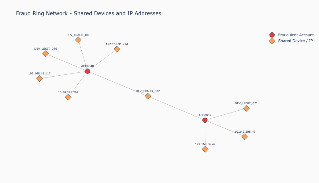
Figure 5-1. Fraud Ring Network Plot.

The fraud ring network plot in Figure 5-1 shows:

• Red circles for fraudulent accounts (ACC0007, ACC0040)
• Orange diamonds for the devices and IP addresses used by the fraudulent accounts
• DEV_FRAUD_002 appears as the central orange diamond connecting the two red nodes - the smoking gun device

The key insight from the visualization is the two-cluster structure. ACC0007 and ACC0040 each have their own satellite devices and IP addresses, but DEV_FRAUD_002 bridges the two clusters. This shared bridge is what a fraud investigator would focus on first.

The device sharing bar chart, shown in Figure 5-2, reinforces this with aggregated data. DEV_FRAUD_002 stands out as a pure red bar - two accounts sharing it, both fraudulent. DEV_LEGIT_071 and DEV_LEGIT_086 show mixed signal with one fraudulent account each - realistic noise that a production system would need to investigate further. All other shared devices are exclusively legitimate.

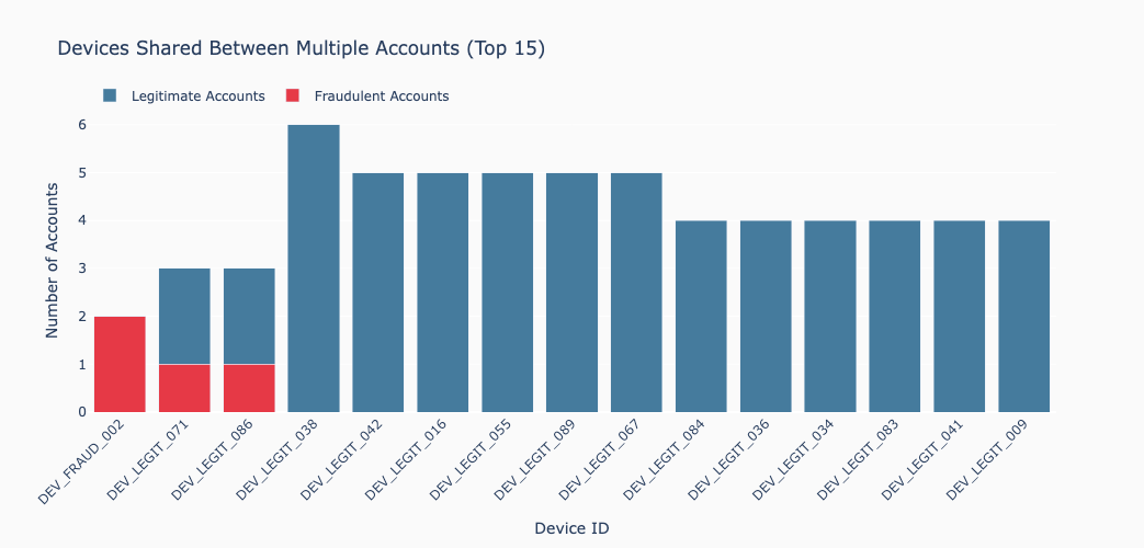
Figure 5-2. Device Sharing.

Fraud ring summary

A final Cypher query aggregates the device sharing pattern across the full dataset:

MATCH (a:Account)-[:MADE]->(t:Transaction)-[:USED_DEVICE]->(d:Device)
WITH d, collect(DISTINCT a) AS accounts
WHERE size(accounts) > 1
RETURN d.device_id AS device_id,
       size(accounts) AS num_accounts,
       size([a IN accounts WHERE a.is_fraud = true]) AS fraud_accounts
ORDER BY fraud_accounts DESC, num_accounts DESC

The notebook prints the first 10 of the 55 devices that more than one account shares (the first two are shown here):

Devices shared between multiple accounts (55 in total, showing the first 10):

  Device: DEV_FRAUD_002
  Accounts: 2 total, 2 fraudulent

  Device: DEV_LEGIT_071
  Accounts: 3 total, 1 fraudulent

DEV_FRAUD_002 rises to the top of the list with 100% fraud rate - a clear signal that any account sharing this device warrants immediate investigation.

What you’d hit in production

Vector search syntax. Newer Neo4j releases deprecate db.index.vector.queryNodes() in favor of the Cypher SEARCH clause. The procedure used in this chapter works correctly, and any deprecation notice can be suppressed via NotificationDisabledCategory.DEPRECATION in the driver configuration. Check the release notes for the version you’re running and plan to move new code to the SEARCH clause.

Loading speed. Inserting each transaction as a separate session call is simple but slow for large datasets. For production bulk loads use UNWIND with batched parameters to insert many nodes and relationships in a single query.

Index creation timing. The vector index must be fully ONLINE before queries will return results. The polling loop using SHOW INDEXES WHERE name = 'index_name' is the reliable way to wait for this - don’t assume the index is ready immediately after the CREATE VECTOR INDEX statement returns.

Combined query result volume. The combined graph and vector search can return a large number of rows when the similarity threshold is low and the graph is densely connected. In production, filter the output to return only connections involving at least one flagged account and consider adding a minimum fraud score threshold to reduce noise.

AuraDB Free tier limits. The free tier has limits on the number of nodes and relationships, on storage and on instances, so check the current limits in the Aura documentation. The dataset in this chapter is well within them. Production fraud detection datasets with millions of transactions and accounts require a paid AuraDB tier or a self-hosted Neo4j Enterprise deployment.

Self-hosted Neo4j. Neo4j can be run locally via Docker or deployed on your own infrastructure. The self-hosted version supports the Graph Data Science (GDS) library, which adds community detection, centrality algorithms and path finding that significantly extend fraud detection capabilities beyond what pure Cypher can express.

When to look elsewhere

Neo4j is the right choice when relationships are central to your problem. Consider alternatives if:

• Your data are not highly connected. If your use case is primarily about finding similar items without traversing networks of entities, a simpler vector database from earlier chapters will serve you better with less operational overhead.
• You need pure vector search at very large scale. Neo4j’s vector index is capable, but purpose-built vector databases are optimized specifically for high-throughput similarity search at hundreds of millions of vectors.
• Your team has no graph database experience. The Cypher query language is learnable, but the graph data modeling mindset - thinking in nodes and relationships rather than tables or documents - requires an adjustment. Factor in the learning curve.
• You need GDS algorithms on a managed cloud service. The AuraDB free tier does not include the Graph Data Science library. If community detection, PageRank or shortest path algorithms are central to your use case, you need either a paid AuraDB tier or a self-hosted deployment.

For problems where the connections between entities are the signal - fraud rings, recommendation networks, knowledge graphs, supply chain analysis - Neo4j offers something the other databases in this book don’t: the ability to combine semantic similarity and graph traversal in a single native query, against a database that was built from the ground up to store and traverse relationships efficiently.

Day 6: Snowflake

What is it?

Snowflake is a leading cloud data platform. It’s where many organizations already store their operational and analytical data - data warehouse exports, CRM records, support tickets, event logs and more. Rather than moving that data to a separate vector database, Snowflake’s native VECTOR data type and VECTOR_COSINE_SIMILARITY function bring vector similarity search directly to the data where it already lives.

This is a different proposition from the previous five days. Snowflake isn’t a vector database - it’s a cloud data warehouse that has added vector search as a first-class capability. The argument is data gravity: if your support tickets, customer records or product data already live in Snowflake, the simplest path to semantic search is to stay there rather than copy data into a dedicated vector system and build a synchronization pipeline to keep the two in sync.

Snowflake’s vector support consists of two main pieces. The VECTOR data type stores fixed-dimension floating-point vectors natively. The VECTOR_COSINE_SIMILARITY function computes cosine similarity between two vectors in a SQL query. Both are available in the trial account used in this chapter.

When would you reach for it?

The clearest signal is existing data in Snowflake. If your organization’s data are already in Snowflake - and for many data engineering and analytics teams it is - adding semantic search is a matter of storing embeddings in a new column and writing a SQL query. There is no new system to provision, no data to move and no synchronization to maintain.

The second signal is a SQL-native team. Data engineers and analysts who already work in Snowflake will find VECTOR_COSINE_SIMILARITY immediately familiar. It slots into existing query patterns, works alongside standard WHERE clauses, GROUP BY aggregations and window functions and integrates naturally with Snowflake’s access control and governance features.

The third signal is analytics alongside search. Snowflake is built for analytical workloads. If your use case requires not just “find similar tickets” but also “how many critical tickets are unresolved this week” and “what is the average resolution time by category”, both questions can be answered in the same database with the same SQL toolchain.

The use case

For this chapter we’ll build a customer support analytics system. Support teams can describe an issue in natural language - “customer cannot log in after forgetting their password” or “application is slow and pages take a long time to load” - and find the most relevant historical tickets from the database. Filters by category, priority and status let teams narrow results to the most actionable matches. A summary analytics query shows ticket volumes and resolution rates by category alongside the semantic search.

This is a natural fit for Snowflake. Support ticket data lives in data warehouses and CRM systems. The people who work with it - support operations, customer success and analytics teams - are SQL users. Adding semantic search without leaving SQL is a meaningful reduction in operational complexity.

The data

We generate synthetic customer support tickets from pools of categories, priorities, products, statuses and description templates. Each ticket has a free-text description and an optional resolution note.

The key fields are:

• TICKET_ID - a unique ticket identifier, e.g. “TKT00042”
• CATEGORY - e.g. “Billing”, “Technical”, “Account”, “Security”
• PRIORITY - “Low”, “Medium”, “High” or “Critical”
• STATUS - “Open”, “In Progress”, “Resolved” or “Closed”
• PRODUCT - one of ten fictional product names
• DESCRIPTION - a prose description of the issue; this is what we embed and search over
• RESOLUTION - a resolution note, present only for resolved and closed tickets
• EMBEDDING - the embedding vector stored as a VARCHAR, cast to VECTOR at query time

Resolution notes are only present for tickets with a status of “Resolved” or “Closed”, which reflects real-world ticket data. This makes resolved tickets particularly useful for finding past solutions to current problems.

Building the application

Prerequisites

To follow along you’ll need:

• A Snowflake free trial account
• Ollama running locally with the all-minilm model pulled
• Python 3.12 with a virtual environment

Note: Snowflake offers a managed vector search service called Cortex Search, which handles embedding generation internally. However, the embedding functions it relies on may not be available on trial accounts, depending on region and account privileges. For this chapter we use Ollama to generate embeddings locally and store them in Snowflake using the native VECTOR data type, which is available on all account types.

Configuration

We’ll set the following environment variables before running the notebook:

export SNOWFLAKE_ACCOUNT="your-account-identifier"
export SNOWFLAKE_USER="your-username"
export SNOWFLAKE_PASSWORD="your-password"

Then in the notebook:

SNOWFLAKE_ACCOUNT   = os.environ["SNOWFLAKE_ACCOUNT"]
SNOWFLAKE_USER      = os.environ["SNOWFLAKE_USER"]
SNOWFLAKE_PASSWORD  = os.environ["SNOWFLAKE_PASSWORD"]
SNOWFLAKE_DATABASE  = "SUPPORT_DB"
SNOWFLAKE_SCHEMA    = "SUPPORT_SCHEMA"
SNOWFLAKE_WAREHOUSE = "SUPPORT_WH"
SNOWFLAKE_ROLE      = "ACCOUNTADMIN"
TABLE_NAME          = "SUPPORT_TICKETS"
LLM_EMBEDDING       = "all-minilm"
NUM_TICKETS         = 200
RANDOM_SEED         = 42

Note: NUM_TICKETS controls the size of the generated dataset. 200 is the recommended default for this chapter - embedding generation runs locally via Ollama and is single-threaded, so larger values will work but will take proportionally longer. Production pipelines would typically use a hosted embedding endpoint with async or batched generation to handle scale.

Determine embedding dimensions

We’ll determine the embedding dimensions dynamically from a test embedding:

def get_embedding(text: str) -> list:
    response = ollama.embeddings(model = LLM_EMBEDDING, prompt = text)
    return response["embedding"]

test_embedding = get_embedding("customer support ticket about billing issue")
EMBEDDING_DIMS = len(test_embedding)
print(f"Embedding dimensions: {EMBEDDING_DIMS}")

Connect to Snowflake

conn = snowflake.connector.connect(
    account  = SNOWFLAKE_ACCOUNT,
    user     = SNOWFLAKE_USER,
    password = SNOWFLAKE_PASSWORD,
    role     = SNOWFLAKE_ROLE,
)

cursor = conn.cursor()
print(f"Connected to Snowflake: {conn.account}")

Create database, schema and warehouse

We’ll create all infrastructure programmatically using cursor.execute(). The warehouse is set to X-SMALL with AUTO_SUSPEND = 60 to minimize credit consumption:

cursor.execute(f"CREATE DATABASE IF NOT EXISTS {SNOWFLAKE_DATABASE}")
cursor.execute(f"USE DATABASE {SNOWFLAKE_DATABASE}")
cursor.execute(f"CREATE SCHEMA IF NOT EXISTS {SNOWFLAKE_SCHEMA}")
cursor.execute(f"USE SCHEMA {SNOWFLAKE_SCHEMA}")
cursor.execute(f"""
    CREATE WAREHOUSE IF NOT EXISTS {SNOWFLAKE_WAREHOUSE}
    WITH WAREHOUSE_SIZE = 'X-SMALL'
    AUTO_SUSPEND = 60
    AUTO_RESUME  = TRUE
""")

cursor.execute(f"USE WAREHOUSE {SNOWFLAKE_WAREHOUSE}")

Generate the dataset

Description templates are category-specific so each ticket gets a relevant, realistic description:

DESCRIPTION_TEMPLATES = {
    "Billing": [
        "Customer was charged twice for the same subscription period and is requesting a refund for the duplicate charge.",
        "Invoice amount does not match the quoted price. Customer is disputing the difference and requesting a corrected invoice.",
        # ... further templates
    ],
    "Technical": [
        "Customer reports the application is crashing on startup after the latest update was applied to their system.",
        "API calls are returning 500 errors intermittently. Customer has provided request IDs and timestamps for investigation.",
        # ... further templates
    ],
    # ... further categories
}

def generate_ticket(ticket_id: int) -> dict:
    category = random.choice(CATEGORIES)
    status   = random.choice(STATUSES)
    return {
        "TICKET_ID":   f"TKT{ticket_id:05d}",
        "CATEGORY":    category,
        "PRIORITY":    random.choice(PRIORITIES),
        "STATUS":      status,
        "PRODUCT":     random.choice(FICTIONAL_PRODUCTS),
        "DESCRIPTION": random.choice(DESCRIPTION_TEMPLATES[category]),
        "RESOLUTION":  RESOLUTION_TEMPLATES[category] if status in ["Resolved", "Closed"] else None,
    }

Generate embeddings

We embed each ticket description locally with Ollama and store the result as a string in a new EMBEDDING column on the DataFrame:

embeddings = []
for ticket in tqdm(tickets, desc = "Generating embeddings"):
    embeddings.append(get_embedding(ticket["DESCRIPTION"]))

df["EMBEDDING"] = [str(e) for e in embeddings]

The embedding is stored as a string because the connector can’t load VECTOR columns directly. We cast it to VECTOR at query time.

Load data into Snowflake

We’ll create the table with an EMBEDDING VARCHAR(16000) column and load the data using write_pandas:

cursor.execute(f"""
    CREATE TABLE {TABLE_NAME} (
        TICKET_ID   VARCHAR(20),
        CATEGORY    VARCHAR(50),
        PRIORITY    VARCHAR(20),
        STATUS      VARCHAR(20),
        PRODUCT     VARCHAR(100),
        DESCRIPTION VARCHAR(1000),
        RESOLUTION  VARCHAR(1000),
        EMBEDDING   VARCHAR(16000)
    )
""")

success, num_chunks, num_rows, _ = write_pandas(
    conn = conn,
    df = df,
    table_name = TABLE_NAME,
    auto_create_table = False
)

Semantic search

We’ll embed the query with Ollama, pass it to Snowflake as a SQL parameter and use VECTOR_COSINE_SIMILARITY to rank results.

Note: Snowflake cannot cast a VARCHAR directly to VECTOR. The stored embedding string must first be parsed into a VARIANT (Snowflake’s JSON type) using TRY_PARSE_JSON, which can then be cast to VECTOR. The same applies to the query embedding passed as a parameter.

def search_tickets(query: str, top_k: int = 5):
    query_embedding = get_embedding(query)
    query_vec_str = str(query_embedding)

    cursor.execute(f"""
        SELECT
            TICKET_ID,
            CATEGORY,
            PRIORITY,
            STATUS,
            PRODUCT,
            DESCRIPTION,
            RESOLUTION,
            VECTOR_COSINE_SIMILARITY(
                TRY_PARSE_JSON(EMBEDDING)::VECTOR(FLOAT, {EMBEDDING_DIMS}),
                TRY_PARSE_JSON(%s)::VECTOR(FLOAT, {EMBEDDING_DIMS})
            ) AS similarity
        FROM {TABLE_NAME}
        ORDER BY similarity DESC
        LIMIT {top_k}
    """, (query_vec_str,))

Sample results (the top two of five are shown):

Query: 'customer cannot log in after forgetting their password'

  TKT00121 | Account | Medium | Open
  Product: AnalyticsDash
  Similarity: 0.714
  Description: Customer has forgotten their password and is not receiving the password reset email in their inbox.

  TKT00088 | Account | Critical | Resolved
  Product: TaskMaster
  Similarity: 0.714
  Description: Customer has forgotten their password and is not receiving the password reset email in their inbox.
  Resolution: Account team verified the customer's identity and restored access. Security review completed.

The two tickets have identical descriptions, so their similarity scores are identical. The generated dataset has only five description templates per category, so ties like this are common. The next three results are two-factor authentication tickets that score 0.492 each, and the order among tied tickets isn’t guaranteed to be the same from one query to the next.

Filtered search

Because the tickets live in a standard Snowflake table, filtering is plain SQL. We’ll add WHERE clauses to the similarity query - no special filter syntax, no filter index declaration, no attribute list defined at index creation time. Any column in the table can be used as a filter:

def search_tickets_filtered(
    query:    str,
    category: str = None,
    priority: str = None,
    status:   str = None,
    product:  str = None,
    top_k:    int = 5
):
    filters = []
    if category: filters.append(f"CATEGORY = '{category}'")
    if priority: filters.append(f"PRIORITY = '{priority}'")
    if status:   filters.append(f"STATUS = '{status}'")
    if product:  filters.append(f"PRODUCT = '{product}'")

    where_clause = "WHERE " + " AND ".join(filters) if filters else ""

    cursor.execute(f"""
        SELECT ...,
            VECTOR_COSINE_SIMILARITY(
                TRY_PARSE_JSON(EMBEDDING)::VECTOR(FLOAT, {EMBEDDING_DIMS}),
                TRY_PARSE_JSON(%s)::VECTOR(FLOAT, {EMBEDDING_DIMS})
            ) AS similarity
        FROM {TABLE_NAME}
        {where_clause}
        ORDER BY similarity DESC
        LIMIT {top_k}
    """, (query_vec_str,))

Finding resolved technical issues is particularly useful for support teams - a query that returns past tickets with resolutions gives agents an immediate starting point for troubleshooting (the top two of four matching tickets are shown):

query = 'API returning errors and integration not working', category = 'Technical', status = 'Resolved'

  TKT00072 | Technical | Critical | Resolved
  Product: InsightEngine
  Similarity: 0.506
  Description: API calls are returning 500 errors intermittently. Customer has provided request IDs and timestamps for investigation.
  Resolution: Engineering team identified the root cause and deployed a fix. Customer confirmed the issue is resolved.

  TKT00034 | Technical | Low | Resolved
  Product: InsightEngine
  Similarity: 0.340
  Description: Integration with a third-party service stopped working after a configuration change on the customer's side.
  Resolution: Engineering team identified the root cause and deployed a fix. Customer confirmed the issue is resolved.

Only four tickets in the dataset are both Technical and Resolved, so the filter returns four results rather than five.

Analytics with SQL

The real advantage of keeping data in Snowflake is the ability to run analytical queries alongside semantic search in the same system. Here we summarize ticket volumes, resolution counts and resolution rates by category:

cursor.execute(f"""
    SELECT
        CATEGORY,
        COUNT(*)                                                            AS TOTAL_TICKETS,
        SUM(CASE WHEN STATUS IN ('Resolved', 'Closed') THEN 1 ELSE 0 END) AS RESOLVED,
        SUM(CASE WHEN PRIORITY = 'Critical' THEN 1 ELSE 0 END) AS CRITICAL,
        ROUND(
            100.0 * SUM(CASE WHEN STATUS IN ('Resolved', 'Closed') THEN 1 ELSE 0 END) / COUNT(*),
            1
        ) AS RESOLUTION_RATE_PCT
    FROM {TABLE_NAME}
    GROUP BY CATEGORY
    ORDER BY TOTAL_TICKETS DESC
""")

summary = cursor.fetch_pandas_all()

No second system, no result merging, no data movement. The semantic search and the analytics live in the same table and run against the same Snowflake warehouse.

What you’d hit in production

Cortex Search on trial accounts. Snowflake Cortex Search handles embedding generation internally and provides a managed search service. However, the underlying embedding functions may not be available on trial accounts, depending on region and account privileges. For production use with a paid Snowflake account, Cortex Search is worth evaluating - it removes the need for an external embedding pipeline and manages index updates as the table changes. For trial accounts or teams with an existing embedding pipeline, the VECTOR + VECTOR_COSINE_SIMILARITY approach shown in this chapter is an alternative.

TRY_PARSE_JSON overhead. Casting the stored VARCHAR to VECTOR via TRY_PARSE_JSON at query time adds overhead compared to storing embeddings natively as VECTOR. For production, consider storing embeddings directly in a VECTOR(FLOAT, N) column rather than as a string. The Snowflake connector can’t load VECTOR columns directly, so you would load the embeddings as an ARRAY into a staging table and cast them into a VECTOR column with an INSERT ... SELECT.

Warehouse costs. Every query that runs VECTOR_COSINE_SIMILARITY across a large table requires the warehouse to be running. With AUTO_SUSPEND = 60, the warehouse suspends after a minute of inactivity. For low-traffic use cases this is cost-effective; for high-traffic search applications the cost of keeping the warehouse running can add up. Cortex Search has its own cost model, so compare the two against your expected query volume.

Full table scan. The VECTOR_COSINE_SIMILARITY query performs a full table scan to compute similarity for every row before sorting and limiting. For datasets of modest size this works well, but query latency grows with the number of rows. Cortex Search is worth evaluating when full scans become too slow.

Warehouse size for large datasets. At 200 tickets an X-SMALL warehouse is more than sufficient. For larger datasets or faster query times, increase the warehouse size. Snowflake scales compute independently of storage, so you can use a larger warehouse for bulk embedding inserts and scale back down for queries.

Snowflake Postgres and pgvector. For applications that need full Postgres semantics alongside Snowflake data, Snowflake Postgres provides a fully managed Postgres with pgvector integrated directly into the platform. See the Snowflake Postgres section below for a working example.

Snowflake Postgres - pgvector inside the data platform

Snowflake Postgres is a fully managed Postgres database integrated directly into the Snowflake platform, available under Manage > Postgres in the Snowflake UI. It’s built on Crunchy Data technology following Snowflake’s acquisition of the company, and brings standard Postgres with pgvector into the data platform context, alongside Snowflake tables, warehouses and governance features.

Unlike the VECTOR_COSINE_SIMILARITY approach used earlier in this chapter, Snowflake Postgres uses the native pgvector <=> cosine distance operator. The connection uses a static password, making it simpler to work with from a notebook.

Prerequisites

Before running the code, create a Snowflake Postgres instance in the Snowflake UI under Manage > Postgres, note the hostname, username and password from the connection string and add your IP address to the network ingress rules. SSL is required for all connections.

Configuration

We’ll set the following environment variables before running the notebook:

export SNOWFLAKE_PG_HOST="your-instance.eu-west-2.aws.postgres.snowflake.app"
export SNOWFLAKE_PG_USER="snowflake_admin"
export SNOWFLAKE_PG_PASSWORD="your-password"
export SNOWFLAKE_PG_DBNAME="postgres"

Then in the notebook:

SNOWFLAKE_PG_HOST     = os.environ["SNOWFLAKE_PG_HOST"]
SNOWFLAKE_PG_USER     = os.environ["SNOWFLAKE_PG_USER"]
SNOWFLAKE_PG_PASSWORD = os.environ["SNOWFLAKE_PG_PASSWORD"]
SNOWFLAKE_PG_DBNAME   = os.environ["SNOWFLAKE_PG_DBNAME"]
SNOWFLAKE_PG_TABLE    = "support_tickets"

Connecting to Snowflake Postgres

Snowflake Postgres uses standard Postgres drivers. We’ll connect with psycopg2 using the static password from the connection string:

pg_conn = psycopg2.connect(
    host     = SNOWFLAKE_PG_HOST,
    user     = SNOWFLAKE_PG_USER,
    password = SNOWFLAKE_PG_PASSWORD,
    dbname   = SNOWFLAKE_PG_DBNAME,
    sslmode  = "require",
    port     = 5432
)

pg_conn.autocommit = True
pg_cursor = pg_conn.cursor()

pgvector on Snowflake Postgres

pgvector is available on Snowflake Postgres and is enabled programmatically in the notebook:

pg_cursor.execute("CREATE EXTENSION IF NOT EXISTS vector;")

Native vector column

Snowflake Postgres supports the native vector type directly. There is no TRY_PARSE_JSON cast required - embeddings are stored and queried as proper vector columns, unlike the VARCHAR approach used with the main Snowflake connector earlier in this chapter:

pg_cursor.execute(f"""
    CREATE TABLE {SNOWFLAKE_PG_TABLE} (
        ticket_id   TEXT PRIMARY KEY,
        category    TEXT,
        priority    TEXT,
        status      TEXT,
        product     TEXT,
        description TEXT,
        resolution  TEXT,
        embedding   VECTOR({EMBEDDING_DIMS})
    )
""")

We’ll reuse the embeddings already generated earlier in the notebook - no additional Ollama calls needed. An HNSW index is created after loading for fast similarity search:

pg_cursor.execute(f"""
    CREATE INDEX ON {SNOWFLAKE_PG_TABLE}
    USING hnsw (embedding vector_cosine_ops)
""")

Queries use the <=> cosine distance operator - identical to Day 1:

def search_snowflake_pg(query: str, top_k: int = 5):
    query_embedding = get_embedding(query)
    pg_cursor.execute(f"""
        SELECT
            ticket_id,
            category,
            priority,
            status,
            product,
            description,
            resolution,
            1 - (embedding <=> %s::vector) AS similarity
        FROM {SNOWFLAKE_PG_TABLE}
        ORDER BY embedding <=> %s::vector
        LIMIT %s
    """, (str(query_embedding), str(query_embedding), top_k))

Sample output (the top result of five):

Snowflake Postgres query: 'customer cannot log in after forgetting their password'

  TKT00121 | Account | Medium | Open
  Product: AnalyticsDash
  Similarity: 0.714
  Description: Customer has forgotten their password and is not receiving
  the password reset email in their inbox.

The top two results match the Snowflake query above, which confirms that both approaches compute the same cosine similarity. Results three to five differ only because tied tickets can come back in any order.

The connection, the vector column and the <=> operator are all standard Postgres and pgvector - the same as Day 1. What has changed is the operational context: the database is fully managed and lives inside the Snowflake platform alongside tables, warehouses and governance features.

When to look elsewhere

Snowflake is the right choice when your data are already there. Consider alternatives if:

• You have no existing Snowflake footprint. Snowflake isn’t free - it operates on a credit model and production usage costs money. Standing up Snowflake just for vector search would be hard to justify when purpose-built vector databases or pgvector on a managed Postgres are simpler and cheaper.
• You need sub-second similarity search at very large scale. Full table scans don’t scale indefinitely. Cortex Search on a paid account addresses this with approximate nearest neighbor indexing, but the approach in this chapter is inherently scan-based.
• Your embedding pipeline isn’t already managed. This chapter requires generating embeddings externally with Ollama and loading them manually. If you’re starting from scratch with no existing pipeline, a database that handles embeddings internally - like Snowflake’s Cortex Search on a paid account - reduces operational complexity.
• Your team isn’t SQL-native. The Snowflake approach is cleanest for teams already working in SQL. For teams building Python applications, the connector-based approach adds friction compared to databases with richer Python SDKs.

For data teams already working in Snowflake, adding vector search to an existing table is a low-friction, high-value addition. The ability to combine semantic search with full SQL analytics in a single system - without moving data or introducing a new operational dependency - is a meaningful advantage for the right team and the right use case.

Day 7: Databricks

What is it?

Databricks is a leading data and AI platform built around the lakehouse architecture - a design that combines the flexibility and scale of a data lake with the structure and governance of a data warehouse. It’s where many data engineering and machine learning teams already store, process and serve their data, using Apache Spark for large-scale computation, Delta Lake for reliable storage and MLflow for experiment tracking.

Databricks SQL adds a familiar SQL interface on top of the lakehouse, letting analysts and data engineers query Delta tables without writing Spark code. The VECTOR_COSINE_SIMILARITY function extends this to vector similarity search over ARRAY<FLOAT> embeddings, making it straightforward to add semantic search to data that already lives in the lakehouse - without introducing a separate vector database.

In 2025 Databricks acquired Neon, a serverless Postgres startup. The acquisition signals Databricks’ intent to extend the lakehouse to cover the full spectrum of database workloads, including the transactional and vector search use cases that Neon’s pgvector support provides. For teams already working in Databricks, this reinforces the “stay in the lakehouse” story that this chapter demonstrates.

When would you reach for it?

The clearest signal is existing data and workflows in Databricks. If your data engineering pipelines, ML experiments and analytical queries already run in Databricks, adding semantic search to a Delta table is a natural extension of what you already do. There’s no new system to learn, no data to move and no synchronization to maintain.

The second signal is a SQL and PySpark team. Data engineers and ML practitioners who work in Databricks already know Delta Lake, Databricks SQL and the Unity Catalog. VECTOR_COSINE_SIMILARITY slots into this existing toolchain as a function call in a familiar SQL query.

The third signal is analytics alongside search. Like Snowflake, Databricks is built for analytical workloads. If your use case requires not just “find the most relevant document” but also “how many documents exist per category” and “how many authors write in each one”, both questions can be answered in the same system with SQL queries.

The use case

For this chapter we’ll build a RAG retrieval layer over internal technical documents - architecture notes, runbooks, API guides, security policies and onboarding materials. Users ask questions in natural language - “how do I restart a service during an incident” or “what are the security requirements for storing sensitive data” - and the system finds the most relevant documents from the corpus.

This is a natural fit for Databricks. Internal technical documentation is exactly the kind of content that data and engineering teams generate, store and share within a data platform. Keeping it searchable in the same system where teams already work reduces friction and keeps governance centralized.

The data

We’ll generate synthetic internal technical wiki documents from pools of categories, authors and content templates. Each document has a title, category, author and a prose content field - the content is what we’ll embed and search over.

The eight categories represent typical internal documentation types:

• Architecture - system design documents and technical overviews
• Runbooks - step-by-step operational procedures for incidents
• API - API reference guides and integration documentation
• Security - access control, data classification and compliance policies
• Onboarding - guides for new team members joining the organization
• Data Engineering - pipeline documentation, data models and ETL guides
• ML Platform - model deployment, feature store and experiment tracking guides
• Incident Reports - post-incident reviews and root cause analyses

The dataset scales via NUM_DOCS. Each document is generated from category-specific templates filled with randomized but realistic-sounding values. Titles and content are filled independently from the same pools, so a title and its content can mention different tasks or systems. All author names are fictional.

Building the application

Prerequisites

To follow along you’ll need:

• A Databricks Free Edition account with access to a SQL warehouse
• Ollama running locally with the all-minilm model pulled
• Python 3.12 with a virtual environment

Generate a personal access token

1. In the Databricks UI, click your username in the top bar and select Settings
2. Click Developer
3. Next to Access tokens, click Manage
4. Click Generate new token, give it a name, select BI Tools as the scope type and click Generate
5. Copy the token immediately, as it’s only shown once

Find your SQL warehouse connection details

1. In the Databricks UI, go to SQL > SQL Warehouses
2. Click your warehouse and select Connection details
3. Note down the Server hostname and HTTP path

Configuration

We’ll set the following environment variables before running the notebook:

export DATABRICKS_SERVER_HOSTNAME="dbc-xxxx.cloud.databricks.com"
export DATABRICKS_HTTP_PATH="/sql/1.0/warehouses/xxxx"
export DATABRICKS_TOKEN="your-personal-access-token"

Then in the notebook:

DATABRICKS_SERVER_HOSTNAME = os.environ["DATABRICKS_SERVER_HOSTNAME"]
DATABRICKS_HTTP_PATH       = os.environ["DATABRICKS_HTTP_PATH"]
DATABRICKS_TOKEN           = os.environ["DATABRICKS_TOKEN"]
CATALOG_NAME               = "workspace"
SCHEMA_NAME                = "wiki_docs"
TABLE_NAME                 = "documents"
LLM_EMBEDDING              = "all-minilm"
NUM_DOCS                   = 200
RANDOM_SEED                = 42

Note: NUM_DOCS controls the size of the generated dataset. 200 is the recommended default for this chapter - embedding generation runs locally via Ollama and is single-threaded, so larger values will work but will take proportionally longer. Production pipelines would typically use a hosted embedding endpoint with async or batched generation to handle scale.

Note: The default catalog in a Free Edition workspace is workspace. If you see a NO_SUCH_CATALOG_EXCEPTION error, check which catalogs are available with SHOW CATALOGS and update CATALOG_NAME accordingly.

Determine embedding dimensions

We’ll determine the embedding dimensions dynamically from a test embedding:

def get_embedding(text: str) -> list:
    response = ollama.embeddings(model = LLM_EMBEDDING, prompt = text)
    return response["embedding"]

test_embedding = get_embedding("internal technical documentation")
EMBEDDING_DIMS = len(test_embedding)
print(f"Embedding dimensions: {EMBEDDING_DIMS}")

Connect to Databricks

conn = sql.connect(
    server_hostname = DATABRICKS_SERVER_HOSTNAME,
    http_path       = DATABRICKS_HTTP_PATH,
    access_token    = DATABRICKS_TOKEN
)

cursor = conn.cursor()
print("Connected to Databricks.")

Generate the dataset

Documents are assembled from category-specific content templates filled with randomized values from component pools. Each category has its own set of templates so the content is relevant to the category:

CONTENT_TEMPLATES = {
    "Architecture": [
        "This document describes the high-level architecture of the {system} platform. "
        "The system is built on a microservices model with {pattern} as the primary "
        "communication pattern. Services are deployed on {infra} and managed via {tool}. "
        "Key design decisions include the use of {decision} to ensure scalability and fault tolerance.",
        # ... further templates
    ],
    "Runbooks": [
        "This runbook covers the procedure for {task} in the {system} environment. "
        "Follow these steps in order during an incident. First, verify the {check} is "
        "responding correctly. If not, escalate to the {team} team and open a P{priority} "
        "incident ticket. Roll back using {rollback} if the issue persists after {timeout} minutes.",
        # ... further templates
    ],
    # ... further categories
}

Generate embeddings

We’ll embed the content of each document locally using Ollama. The embedding is stored as a string and cast to ARRAY<FLOAT> at query time:

embeddings = []
for doc in tqdm(documents, desc = "Generating embeddings"):
    embeddings.append(get_embedding(doc["CONTENT"]))

df["EMBEDDING"] = [str(e) for e in embeddings]

Load data into Databricks

We’ll create a Delta table and load all documents in a single bulk INSERT. The embedding is stored as a STRING column holding JSON text, for reasons explained below.

Note: Inserting one row per document over a network connection to Databricks is extremely slow - each cursor.execute() call is a separate round trip. Concatenating all rows into a single VALUES clause and sending one SQL statement is significantly faster.

values = []
for i, doc in enumerate(documents):
    embedding_str = json.dumps(embeddings[i])
    title    = doc["TITLE"].replace("'", "\\'")
    category = doc["CATEGORY"].replace("'", "\\'")
    author   = doc["AUTHOR"].replace("'", "\\'")
    content  = doc["CONTENT"].replace("'", "\\'")
    emb      = embedding_str.replace("'", "\\'")
    values.append(
        f"('{doc['DOC_ID']}', '{title}', '{category}', '{author}', '{content}', '{emb}')"
    )

cursor.execute(f"""
    INSERT INTO {CATALOG_NAME}.{SCHEMA_NAME}.{TABLE_NAME}
    (DOC_ID, TITLE, CATEGORY, AUTHOR, CONTENT, EMBEDDING)
    VALUES {', '.join(values)}
""")

Note that single quotes in text fields must be escaped before interpolation into the SQL string.

Semantic search

We’ll embed the query with Ollama and pass it to Databricks SQL as a parameter. VECTOR_COSINE_SIMILARITY computes cosine similarity between the stored embedding and the query embedding.

Note: VECTOR_COSINE_SIMILARITY operates on ARRAY<FLOAT> values. We store the embeddings as JSON text in a STRING column, which keeps the bulk INSERT simple, and FROM_JSON parses the text into an ARRAY<FLOAT> at query time. Both the stored embedding and the query embedding need this parsing step.

def search_docs(query: str, top_k: int = 5):
    query_embedding = get_embedding(query)
    query_json      = json.dumps(query_embedding)

    cursor.execute(f"""
        SELECT
            DOC_ID,
            TITLE,
            CATEGORY,
            AUTHOR,
            CONTENT,
            VECTOR_COSINE_SIMILARITY(
                FROM_JSON(EMBEDDING, 'ARRAY<FLOAT>'),
                FROM_JSON(?, 'ARRAY<FLOAT>')
            ) AS similarity
        FROM {CATALOG_NAME}.{SCHEMA_NAME}.{TABLE_NAME}
        ORDER BY similarity DESC
        LIMIT {top_k}
    """, (query_json,))

Sample results (top two of five):

Query: 'how do I restart a service during an incident'

  DOC00108 | Runbooks | Reese Fontaine
  Title: ReportingService Operations Guide
  Similarity: 0.553
  Content: This runbook covers the procedure for restarting the service in the EventBus environment. Follow these steps in order during an incident. First, verif...

  DOC00039 | Runbooks | Casey Petrov
  Title: Runbook: database connection exhaustion in EventBus
  Similarity: 0.508
  Content: This runbook documents the steps to restarting the service for the DataVault service. Prerequisites: access to the admin panel. Steps: (1) Verify aler...

Filtered search

Because the documents live in a standard Delta table, filtering is plain SQL. Any column in the table can be used as a filter - no attribute declaration, no separate filter index:

def search_docs_filtered(
    query:    str,
    category: str = None,
    author:   str = None,
    top_k:    int = 5
):
    filters = []
    if category: filters.append(f"CATEGORY = '{category}'")
    if author:   filters.append(f"AUTHOR = '{author}'")

    where_clause = "WHERE " + " AND ".join(filters) if filters else ""

    cursor.execute(f"""
        SELECT ...,
            VECTOR_COSINE_SIMILARITY(
                FROM_JSON(EMBEDDING, 'ARRAY<FLOAT>'),
                FROM_JSON(?, 'ARRAY<FLOAT>')
            ) AS similarity
        FROM {CATALOG_NAME}.{SCHEMA_NAME}.{TABLE_NAME}
        {where_clause}
        ORDER BY similarity DESC
        LIMIT {top_k}
    """, (query_json,))

Filtering to runbooks during an incident gives an immediately useful result set (top two of five):

query = 'steps to roll back a failed deployment', category = 'Runbooks'

  DOC00024 | Runbooks | Jordan Blake
  Title: AnalyticsAPI Runbook: scaling the cluster
  Similarity: 0.574
  Content: This runbook covers the procedure for rolling back a deployment in the SearchEngine environment. Follow these steps in order during an incident. First...

  DOC00138 | Runbooks | Riley Kumar
  Title: Runbook: high error rates in DataVault
  Similarity: 0.547
  Content: This runbook covers the procedure for rolling back a deployment in the DataVault environment. Follow these steps in order during an incident. First, v...

The first title says “scaling the cluster” while the content is about rolling back a deployment. That’s the independent title and content filling described earlier, not a search error.

Analytics with SQL

The analytics query uses a window function to compute each category’s share of the total document corpus alongside absolute counts:

cursor.execute(f"""
    SELECT
        CATEGORY,
        COUNT(*) AS TOTAL_DOCS,
        COUNT(DISTINCT AUTHOR) AS UNIQUE_AUTHORS,
        ROUND(100.0 * COUNT(*) / SUM(COUNT(*)) OVER (), 1) AS PCT_OF_TOTAL
    FROM {CATALOG_NAME}.{SCHEMA_NAME}.{TABLE_NAME}
    GROUP BY CATEGORY
    ORDER BY TOTAL_DOCS DESC
""")

No second system, no result merging, no data movement. The semantic search and the analytics run against the same Delta table in the same Databricks SQL warehouse.

What you’d hit in production

Free Edition usage limits. Databricks Free Edition runs on serverless compute with a usage quota. The quota can be used up quickly if you run large queries repeatedly.

FROM_JSON overhead. Parsing a STRING into an ARRAY<FLOAT> via FROM_JSON adds overhead for every row on every query. For production, store the embeddings in an ARRAY<FLOAT> column and convert them once at load time. The FROM_JSON approach is reliable and readable but isn’t optimal for very large tables.

Full table scan. Every query parses the stored embedding and computes the similarity for every row before sorting and limiting. For datasets with hundreds of thousands of documents this will become slow. Databricks Vector Search uses approximate nearest neighbor indexing to avoid this, but check whether it’s available on your plan. On Free Edition, keeping the dataset to a smaller number of documents is a practical limit.

Databricks Vector Search. Databricks also offers a managed Vector Search service backed by Delta tables, with approximate nearest neighbor indexing and automatic sync as the underlying table changes. Availability depends on your plan. This is the production path for large-scale semantic search in Databricks and avoids the full scan limitation entirely. The approach in this chapter demonstrates the same concept with standard SQL functions as a starting point.

Bulk insert limit. The single-statement bulk insert approach works well for datasets up to a few hundred documents. For larger datasets the SQL string becomes very large and may hit connector or warehouse limits. For production bulk loads, use Databricks’ native data ingestion tools such as COPY INTO or the Auto Loader, which are designed for large-scale data movement into Delta tables.

Lakebase and pgvector. For production RAG applications that need low-latency reads and full Postgres semantics alongside lakehouse data, Databricks Lakebase provides a fully managed Postgres with pgvector integrated directly into the platform. See the Lakebase section below for a working example.

Lakebase - pgvector inside the Lakehouse

Databricks Lakebase is a fully managed Postgres database integrated directly into the Databricks platform. It’s the product of Databricks’ acquisition of Neon in 2025 and brings serverless Postgres with pgvector into the lakehouse context, with scale-to-zero compute.

This is significant for the book’s story. Day 1 started with pgvector on a local Postgres install. Day 7 ends with pgvector running inside the Databricks lakehouse as a fully managed service. The underlying technology is the same; the operational context is completely different.

Configuration

We’ll set the following environment variables before running the notebook:

export LAKEBASE_HOST="ep-xxxx.database.xxxx.cloud.databricks.com"
export LAKEBASE_USER="your-email-address"
export LAKEBASE_TOKEN="your-oauth-token"
export LAKEBASE_DBNAME="databricks_postgres"

Then in the notebook:

LAKEBASE_HOST   = os.environ["LAKEBASE_HOST"]
LAKEBASE_USER   = os.environ["LAKEBASE_USER"]
LAKEBASE_TOKEN  = os.environ["LAKEBASE_TOKEN"]
LAKEBASE_DBNAME = os.environ["LAKEBASE_DBNAME"]
LAKEBASE_TABLE  = "wiki_documents"

Connecting to Lakebase

Lakebase uses standard Postgres drivers. We’ll connect with psycopg2 using an OAuth token obtained from the Lakebase Connect dialog in the Databricks UI:

lb_conn = psycopg2.connect(
    host     = LAKEBASE_HOST,
    user     = LAKEBASE_USER,
    password = LAKEBASE_TOKEN,
    dbname   = LAKEBASE_DBNAME,
    sslmode  = "require",
    port     = 5432
)

Note: The OAuth token expires after one hour. For production use, the recommended approach is OAuth token rotation via a Databricks service principal and the generate_database_credential() method from the Databricks SDK, which generates a fresh token for each new connection automatically.

pgvector on Lakebase

pgvector is available on Lakebase and is enabled programmatically in the notebook:

lb_cursor.execute("CREATE EXTENSION IF NOT EXISTS vector;")

Native vector column

Unlike the Delta table approach earlier in this chapter, Lakebase supports the pgvector VECTOR type directly. There’s no FROM_JSON cast required - embeddings are stored and queried as proper vector columns:

lb_cursor.execute(f"""
    CREATE TABLE {LAKEBASE_TABLE} (
        doc_id    TEXT PRIMARY KEY,
        title     TEXT,
        category  TEXT,
        author    TEXT,
        content   TEXT,
        embedding VECTOR({EMBEDDING_DIMS})
    )
""")

We’ll reuse the embeddings already generated earlier in the notebook - no additional Ollama calls needed. An HNSW index is created after loading for fast similarity search:

lb_cursor.execute(f"""
    CREATE INDEX ON {LAKEBASE_TABLE}
    USING hnsw (embedding vector_cosine_ops)
""")

Queries use the <=> cosine distance operator - identical to Day 1:

lb_cursor.execute(f"""
    SELECT
        doc_id, title, category, author, content,
        1 - (embedding <=> %s::vector) AS similarity
    FROM {LAKEBASE_TABLE}
    ORDER BY embedding <=> %s::vector
    LIMIT %s
""", (str(query_embedding), str(query_embedding), top_k))

Sample output (top result of five):

Lakebase query: 'how do I restart a service during an incident'

  DOC00108 | Runbooks | Reese Fontaine
  Title: ReportingService Operations Guide
  Similarity: 0.553
  Content: This runbook covers the procedure for restarting the service in the EventBus environment. Follow these steps in order during an incident. First, verif...

All five results and their scores are identical to the Delta table search earlier in the chapter, which is a useful cross-check that both approaches compute the same cosine similarity.

The Lakebase connection, the vector column and the <=> operator are all standard Postgres and pgvector - the same as Day 1. What has changed is the operational context: the database is fully managed, scales to zero when idle and lives inside the Databricks platform alongside Delta tables, ML models and pipelines.

When to look elsewhere

Databricks is the right choice when your data and workflows already live there. Consider alternatives if:

• You have no existing Databricks footprint. Databricks is a commercial platform and standing it up just for vector search is hard to justify when simpler options exist. Day 1 (pgvector) and Day 3 (Pinecone) are considerably easier starting points.
• You need sub-second semantic search at large scale. The full table scan approach in this chapter doesn’t scale to millions of documents at interactive latency. Databricks Vector Search addresses this with approximate nearest neighbor indexing, but it’s a separate service to set up.
• Your team is not already working in SQL or PySpark. The Databricks connector-based approach adds friction compared to databases with richer Python SDKs designed for application developers.
• You need the embedding pipeline to be fully managed. This chapter generates embeddings locally with Ollama. Databricks does offer managed embedding models through its Foundation Model APIs, and using them would remove the external embedding step.

For data and ML teams already living in Databricks, adding semantic search to a Delta table is a natural and low-friction extension of existing workflows. The ability to combine document retrieval with full analytical SQL in a single system - without moving data or managing a separate vector service - makes Databricks a compelling choice for the right team.

Conclusions

What we built

Over seven days we built seven working applications, each demonstrating vector similarity search in a different database against a different use case. We searched job listings, found recipes, searched electronics products, discovered research papers, detected fraud, analyzed support tickets and retrieved internal documents. Every example used the same embedding model, the same general chapter structure and the same honest framing: here is what this database is genuinely good at and here is when you should look elsewhere.

The notebooks are real. The gotchas are real. The “when to look elsewhere” sections are meant. This isn’t a marketing guide.

What we learned

The right database depends on where your data already lives

The most consistent theme across all seven chapters is data gravity. The best vector database for your use case is often the one that already holds your data.

If your application runs on Postgres, pgvector is one command away. If your data are in MongoDB, Atlas Vector Search is a field on your existing documents. If your analytics team lives in Snowflake or Databricks, VECTOR_COSINE_SIMILARITY is a SQL function call. Adding a dedicated vector database to a stack that already has one of these systems means synchronization, dual writes and operational overhead. That overhead is only justified if the dedicated system offers something genuinely unavailable in what you already have.

Purpose-built databases earn their place at scale and in specific scenarios

Pinecone’s managed simplicity is real. Weaviate’s hybrid search - the ability to blend BM25 keyword matching with vector similarity in a single alpha parameter - is genuinely differentiated for knowledge-heavy retrieval. Neo4j’s ability to combine graph traversal with vector search in a single Cypher query is something none of the other databases in this book does natively.

These capabilities matter when they’re the right fit. Pure-play vector search at hundreds of millions of vectors, hybrid search over technical content where exact terminology matters, fraud ring detection where relationships between entities are the signal - these are the scenarios where a purpose-built system earns its complexity.

Vector search and relational filtering are natural partners

Across all seven chapters, the most compelling demonstrations weren’t the pure vector searches but the filtered ones. Semantic similarity combined with structured constraints - category, salary, publication year, priority, fraud status - is more useful than either alone. Every database in this book handles this combination, but in different ways and with different trade-offs.

Postgres and SQL-native systems handle it most naturally because the filter is just a WHERE clause. MongoDB Atlas and Pinecone apply the filter as part of the search itself, which produces better results when filters are selective. Atlas needs the filter fields declared in the index definition, while Pinecone filters on the metadata stored with each record. Weaviate accepts any property in the collection schema as a filter, with no separate declaration. Understanding which approach a database uses matters when your filters are highly selective.

Gotchas are part of the story

Every chapter encountered real friction. pgvector had to be installed from source on Apple Silicon. MongoDB Atlas reports an index as ready before queries will actually return results. Pinecone’s free tier is limited to a single AWS region, us-east-1. Weaviate’s free tier supports only the hfresh index type, not HNSW. Neo4j’s db.index.vector.queryNodes() procedure is deprecated in favor of the Cypher SEARCH clause, which is still a preview feature. Snowflake Cortex Search may not be available on trial accounts, depending on region and account privileges. Databricks SQL has no native vector type, so we stored embeddings as JSON text and parsed them with FROM_JSON at query time.

These aren’t edge cases. They’re the real experience of setting up these systems for the first time and documenting them honestly is one of the things that makes this book useful rather than just promotional.

pgvector is everywhere

One observation that cuts across the whole book: pgvector has spread far beyond standalone Postgres. It powers Databricks Lakebase, which came from the Neon acquisition. It’s available in Snowflake Postgres, which is built on Crunchy Data technology, and in managed Postgres offerings such as Supabase. The book starts with pgvector on a local Mac install and ends with pgvector running inside the Databricks lakehouse as a fully managed service. The underlying technology is the same. The operational context has changed completely.

Choosing the right database

Rather than a ranking, here is a practical decision guide based on what we learned across the seven chapters:

Start with what you have. If you’re already running Postgres, MongoDB, Snowflake or Databricks, try adding vector search there first. The operational simplicity argument is strong and the capabilities are sufficient for most use cases.

Reach for Pinecone when simplicity is the priority. If your use case is pure similarity search with metadata filtering and you want zero infrastructure overhead, Pinecone’s managed service is hard to beat. The data model is minimal by design.

Reach for Weaviate when keywords matter alongside meaning. If your users search for specific technical terms as well as concepts, hybrid search with a tunable alpha parameter is a meaningful capability. Weaviate is also an open-source option if self-hosting matters.

Reach for Neo4j when connections are the signal. If the interesting questions in your domain involve networks of entities - fraud rings, recommendation graphs, knowledge graphs, supply chains - graph traversal combined with vector search is a capability that relational and document databases can only approximate.

Stay in the data platform when your data are already there. For Snowflake and Databricks users, VECTOR_COSINE_SIMILARITY brings semantic search to existing tables without new infrastructure. The full-scan limitation is real but manageable at the scales where teams are typically starting out.

What comes next

The vector database landscape is moving quickly. Several things will have changed by the time you read this:

Cortex Search may become available on more Snowflake accounts, which would remove the trial account limitation described on Day 6.

Databricks Lakebase is actively developing. The Neon acquisition has produced a fully managed Postgres with pgvector integrated into the lakehouse. How deeply it integrates with Delta Lake and Unity Catalog will shape whether it becomes the default choice for Databricks teams that need vector search.

Embedding models are improving rapidly. The all-minilm model we used throughout this book is fast and free but not state of the art. Production systems should evaluate embedding quality as carefully as they evaluate the database.

Approximate nearest neighbor algorithms continue to improve. HNSW is currently the default for most systems, but research into better index structures is active and the landscape may shift.

The databases themselves will also evolve. Weaviate’s free tier may gain HNSW support. Neo4j’s SEARCH clause will move from preview to general availability. Pinecone will add capabilities. MongoDB will refine its pre-filtering model. The specific gotchas in this book will become outdated; the underlying evaluation framework will not.

A final note

The goal of this book wasn’t to pick a winner. It was to give you enough honest, hands-on experience with seven different approaches that you can make a good decision for your own situation. Vector search isn’t a feature you bolt on - it’s an architectural choice that affects your data model, your query patterns, your operational overhead and your costs.

The best database for your use case is the one that fits your data, your team and your scale. We hope this book has made that choice a little clearer.

Free Books

The SingleStore Cookbook: Recipes for Multi-Model, Machine Learning and AI Data Engineering

Read Online ↗

A hands-on cookbook covering SingleStore’s multi-model capabilities, from time series and geospatial data through vector search, machine learning pipelines and AI-powered applications. The recipes draw on first-hand experience building applications with the platform and are organized into four parts:

1. Multi-Model
2. Streaming and Big Data Pipelines
3. Machine Learning
4. AI and Agentic Frameworks

Seven Vector Databases in Seven Days

Read Online ↗

A practical guide that takes one vector database per day and pairs each with a use case chosen to showcase that database’s strengths. Databases covered:

1. PostgreSQL and pgvector - Semantic job search
2. MongoDB Atlas - Recipe finder
3. Pinecone - E-commerce search
4. Weaviate - Research paper discovery
5. Neo4j - Fraud detection
6. Snowflake - Customer support analytics
7. Databricks - RAG over internal documents

Each chapter is self-contained, comes with a Jupyter notebook and gives an assessment of when you’d look elsewhere.

Generative AI: A Manager’s Guide

Read Online ↗

A practical guide for managers, directors and executives who need to make decisions about AI in their organizations, not the engineers building it, but the people responsible for making it work well. The book uses a single central metaphor, the Digital Intern, to frame what AI is genuinely good at, where it falls short and what managing it actually requires. It covers governance, risk, board-level accountability, business case building and the organizational change of moving from pilot to embedded capability.

Seven Ways to Do Vector Search in Python

Read Online ↗

A practitioner’s guide that benchmarks seven Python libraries against the same dataset, measuring recall and latency consistently so you can compare like-for-like. Libraries covered:

1. FAISS
2. Voyager
3. Scikit-learn NearestNeighbors
4. PyNNDescent
5. USearch
6. Chroma
7. LanceDB

Each chapter covers one library, explains what it’s genuinely good at and when you’d reach for something else.

Real-Time Vehicle Tracking with Neo4j, Databricks Lakebase and OpenStreetMap

Read Online ↗

A fleet operations demo that puts ten simulated vehicles onto real road networks loaded from OpenStreetMap. The architecture:

• Neo4j Aura holds the road network graph
• Databricks Lakebase stores live vehicle positions
• Databricks Lakehouse handles historical analytics

Two Streamlit dashboards display live positions and trend data. The primary demo uses the London Borough of Merton, with additional configurations for San Francisco and Singapore.

Real-Time Supply Chain Routing with Neo4j, Snowflake Postgres and Confluent Kafka

Read Online ↗

A supply chain routing demo that combines graph-based route optimization with real-time event streaming. The architecture:

• Neo4j Aura holds the supplier and logistics network graph
• Snowflake Postgres stores product and inventory data
• Confluent Kafka streams supply chain events in real time

Route queries traverse the graph to find optimal paths between suppliers, warehouses and distribution centers under live capacity and disruption constraints.

Neo4j Beyond the Graph

Read Online ↗

A hands-on guide to Neo4j’s multi-model capabilities, going beyond graph traversal to explore seven native features of the platform. Each chapter pairs one capability with a use case chosen to showcase it:

1. Native Graph - London Underground routing
2. Full-Text Search - Research paper discovery
3. Geospatial - Air quality along the Pyrenees corridor
4. Temporal - S&P 500 stock price analysis
5. Document-Style Properties - Library inventory management
6. Vector Search - Fashion image similarity
7. Graph + Vector - Fraud ring detection

Every chapter comes with a Jupyter notebook and a Streamlit application. All examples run on Neo4j Aura’s free tier.

Seven Ways to Use Jev

Read Online ↗

A practical guide to TypeSafe AI’s structured decision model, exploring seven domains where a single Choice call – structured state in, typed decision out, calibrated confidence alongside – replaces brittle rules-based logic. Each chapter pairs one domain with a hands-on Jupyter notebook and examines what the confidence score reveals about the decision:

1. Transit Routing - Northern Line branch triage using a NetworkX graph
2. Customer Support Triage - Ticket routing by team and priority
3. Financial Fraud Detection - Flag or pass with a three-tier confidence response
4. Content Moderation - Approve, flag or remove user-generated content
5. Supply Chain Disruption - Alternative supplier selection under live constraints
6. Hiring Screening - CV screening against a structured job description
7. Medical Symptom Triage - Care pathway assignment with a conservative bias

A recurring theme across all seven chapters: the confidence score is more informative than the decision itself for uncertain cases and the threshold between automatic routing and human review is always a business decision, not a technical one.

Lessons Learned Putting Jev Inside Neo4j

Read Online ↗

A hands-on account of building a Neo4j function and batch procedure in Java that ask a model to make a decision about a node and store the answer back in the graph. The book follows one running example, 500 synthetic transactions and each chapter adds the code that the previous chapter’s problem called for. The lessons:

1. Why in the Database - Where a decision belongs and what the finished function returns
2. A First Working Function - Converting Neo4j’s types on the way in and out
3. Failures as Data - Returning errors as values so one bad node can’t stop a query
4. Testing Without a Network - Seams for the network and the clock, with 68 fast tests
5. Keeping the Key Safe - Sending a credential only to the host the parser reports
6. Many at Once - A bounded, ordered pool and a measured concurrency sweep
7. Running It Locally - Swapping in a small local model and seeing how the judgment changes

Every chapter with code has its own folder in the repository and each Cypher script also comes as a notebook, so you can use whichever you prefer. The results are reported as measured, including the ones we can’t explain!